


-
摘要:
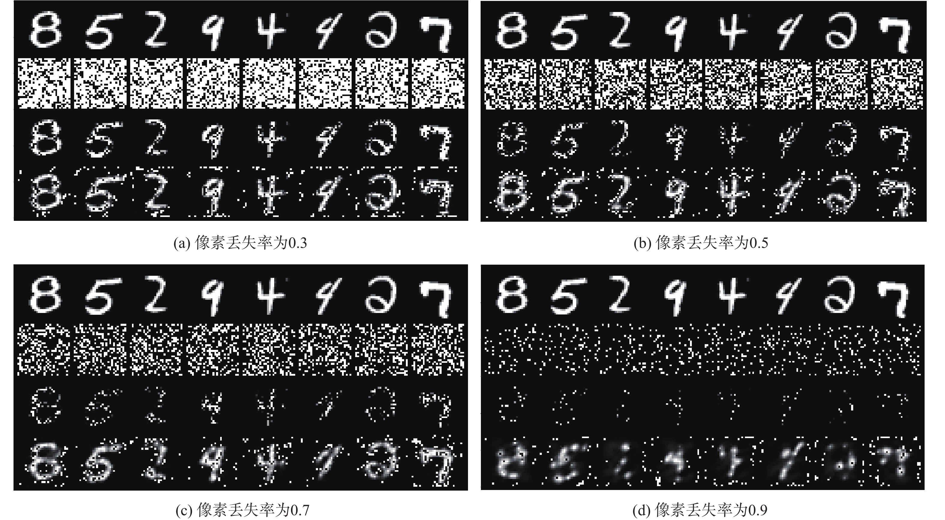
神经随机微分方程模型(SDE-Net)可以从动力学系统的角度来量化深度神经网络(DNNs)的认知不确定性。但SDE-Net面临2个问题,一是在处理大规模数据集时,随着网络层次的增加会导致性能退化;二是SDE-Net在处理具有噪声或高丢失率的分布内数据所引起的偶然不确定性问题时性能较差。为此设计了一种残差SDE-Net(ResSDE-Net),该模型采用了改进的残差网络(ResNets)中的残差块,并应用于SDE-Net以获得一致稳定性和更高的性能;针对具有噪声或高丢失率的分布内数据,引入具有平移等变性的卷积条件神经过程 (ConvCNPs)进行数据修复,从而提高ResSDE-Net处理此类数据的性能。实验结果表明:ResSDE-Net在处理分布内和分布外的数据时获得了一致稳定的性能,并在丢失了70%像素的MNIST、CIFAR10及实拍的SVHN数据集上,仍然分别获得89.89%、65.22%和93.02%的平均准确率。
Abstract:The neural stochastic differential equation model (SDE-Net) can quantify epistemic uncertainties of deep neural networks (DNNs) from the perspective of a dynamical system. However, SDE-Net faces two problems. Firstly, when dealing with largescale datasets, performance degrades as network layers increase. Secondly, SDE-Net has poor performance in dealing with aleatoric uncertainties caused by in-distribution data with noise or a high missing rate. In order to achieve consistent stability and higher performance, this paper first designs a residual SDE-Net (ResSDE-Net) model, which enhances the residual blocks in residual networks (ResNets). next, convolutional conditional neural processes (ConvCNPs) with translation equivariance are introduced to complete in-distribution data that has noise or a high rate of missing data in order to enhance the ResSDE-Net's processing ability for such datasets. The experimental results demonstrate that the ResSDE-Net performs consistently and predictably when dealing with in-distribution and out-of-distribution data. Additionally, the model still achieves an average accuracy of 89.89%, 65.22%, and 93.02% on the real-world SVHN datasets and the MNIST, CIFAR10, and CIFAR10 datasets, where 70% of the pixels are lost, respectively.
-
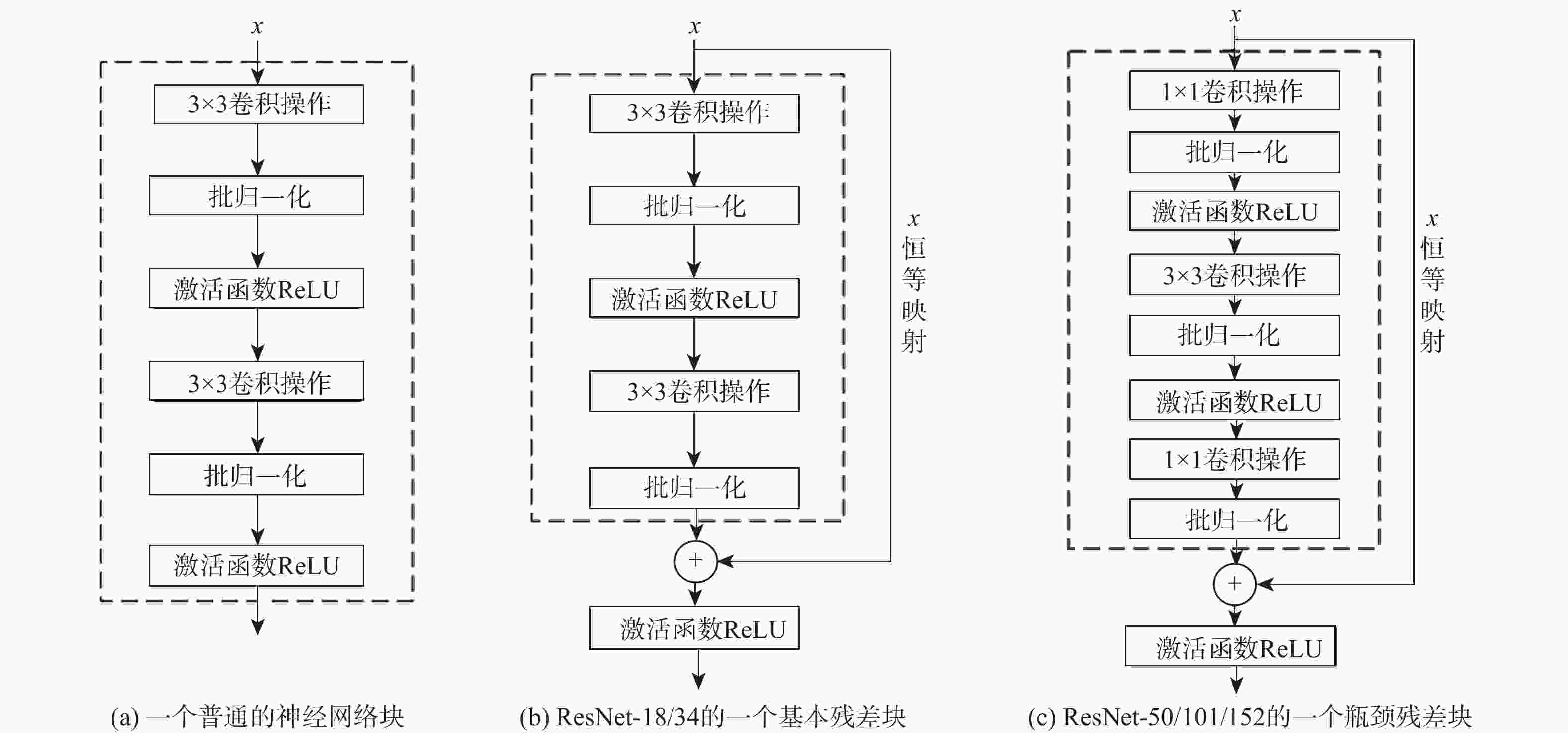
图 1 普通神经网络、基本残差块或瓶颈残差块所构建的DNNs
Figure 1. DNNs constructed with plain networks, basic or bottleneck residual block

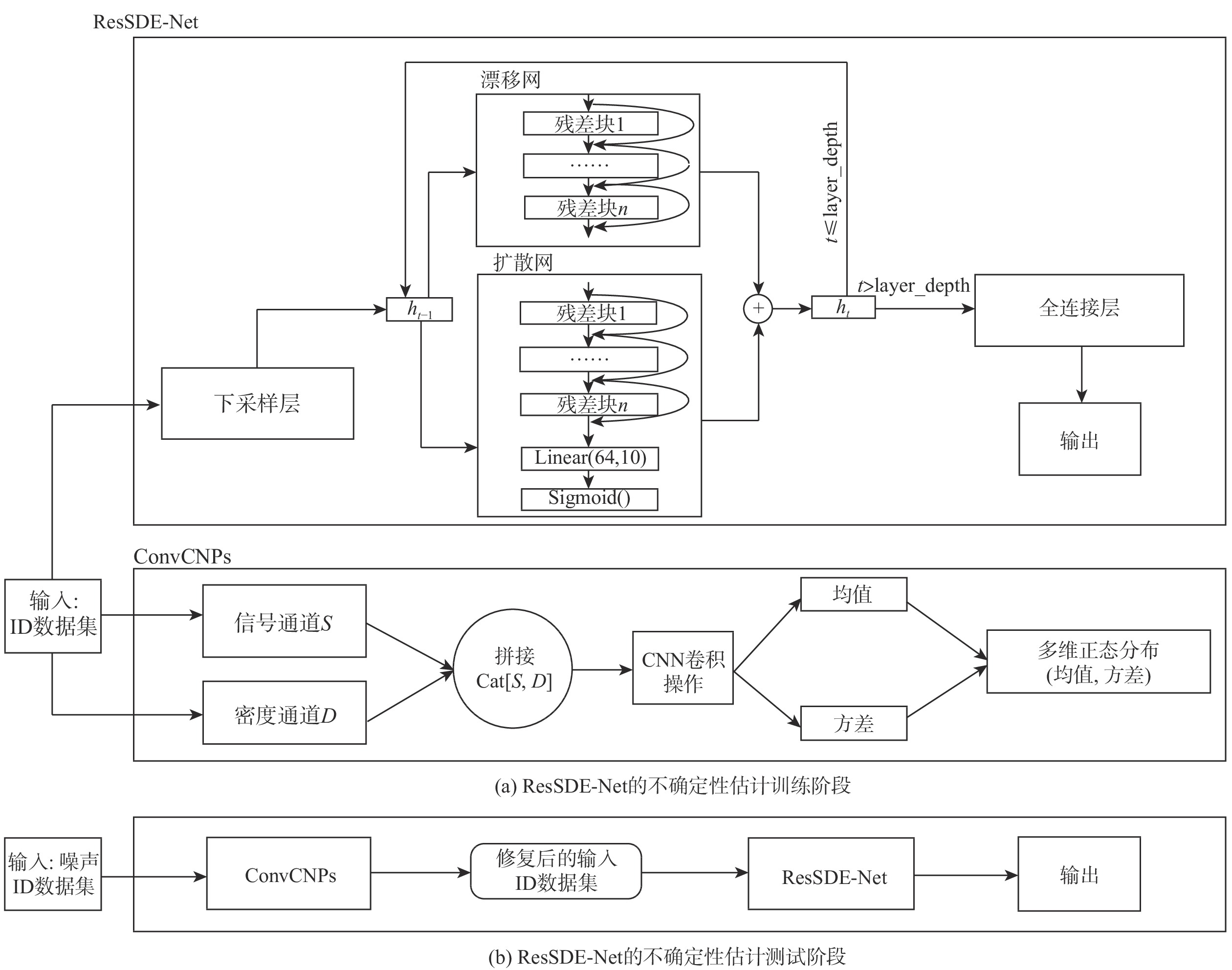
图 2 用于训练和测试阶段的ResSDE-Net的不确定性估计方法框架
Figure 2. Framework for the uncertainty estimates of the proposed ResSDE-Net for training and testing phases

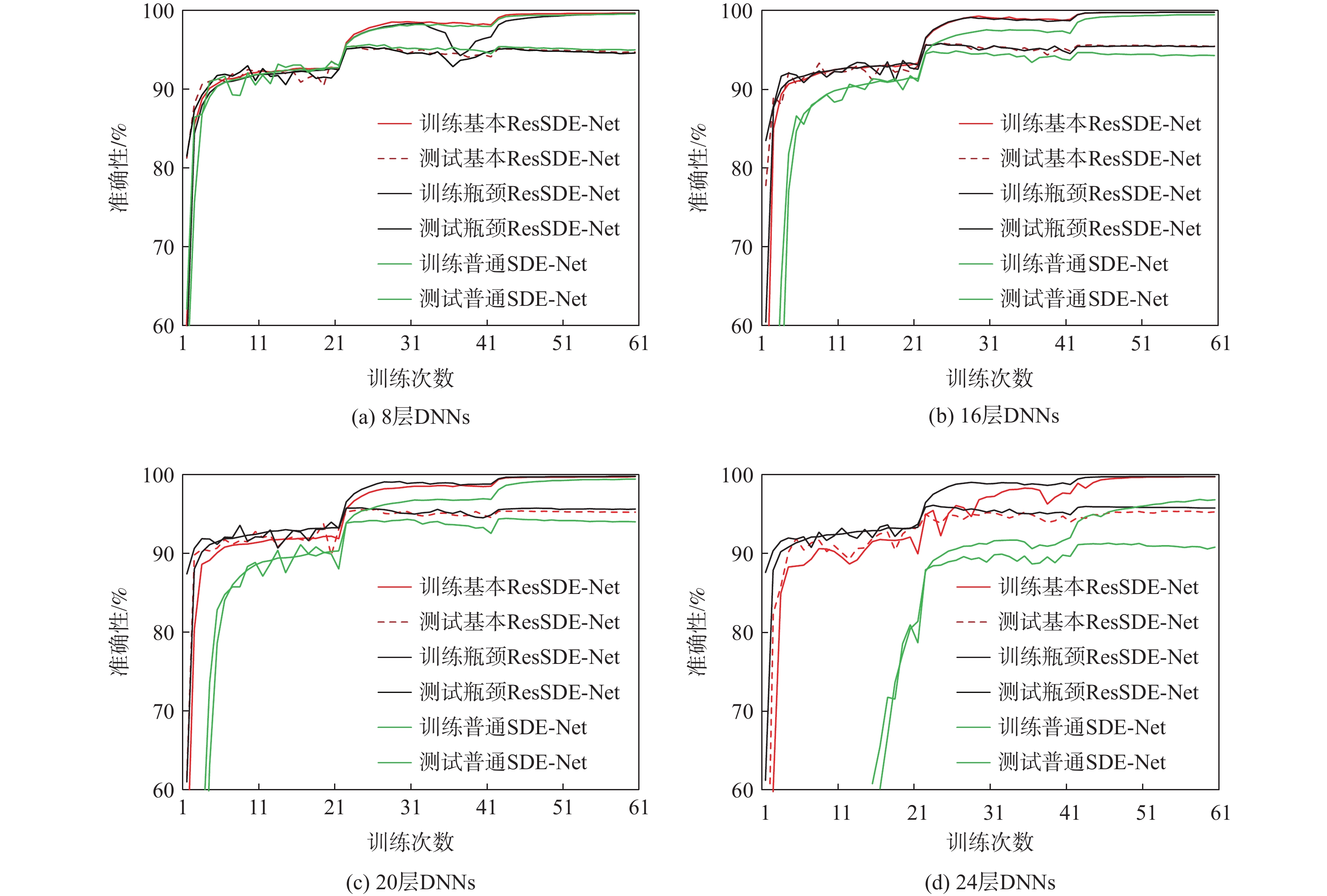
图 3 具有8/16/20/24层DNNs的SDE-Net由基本残差块、瓶颈残差块和普通块所构建模型的训练和测试准确性结果
Figure 3. Training and testing accuracy results of SDE-Net with basic residual blocks, bottleneck residual blocks and plain building blocks to construct 8/16/20/24-layer DNNs
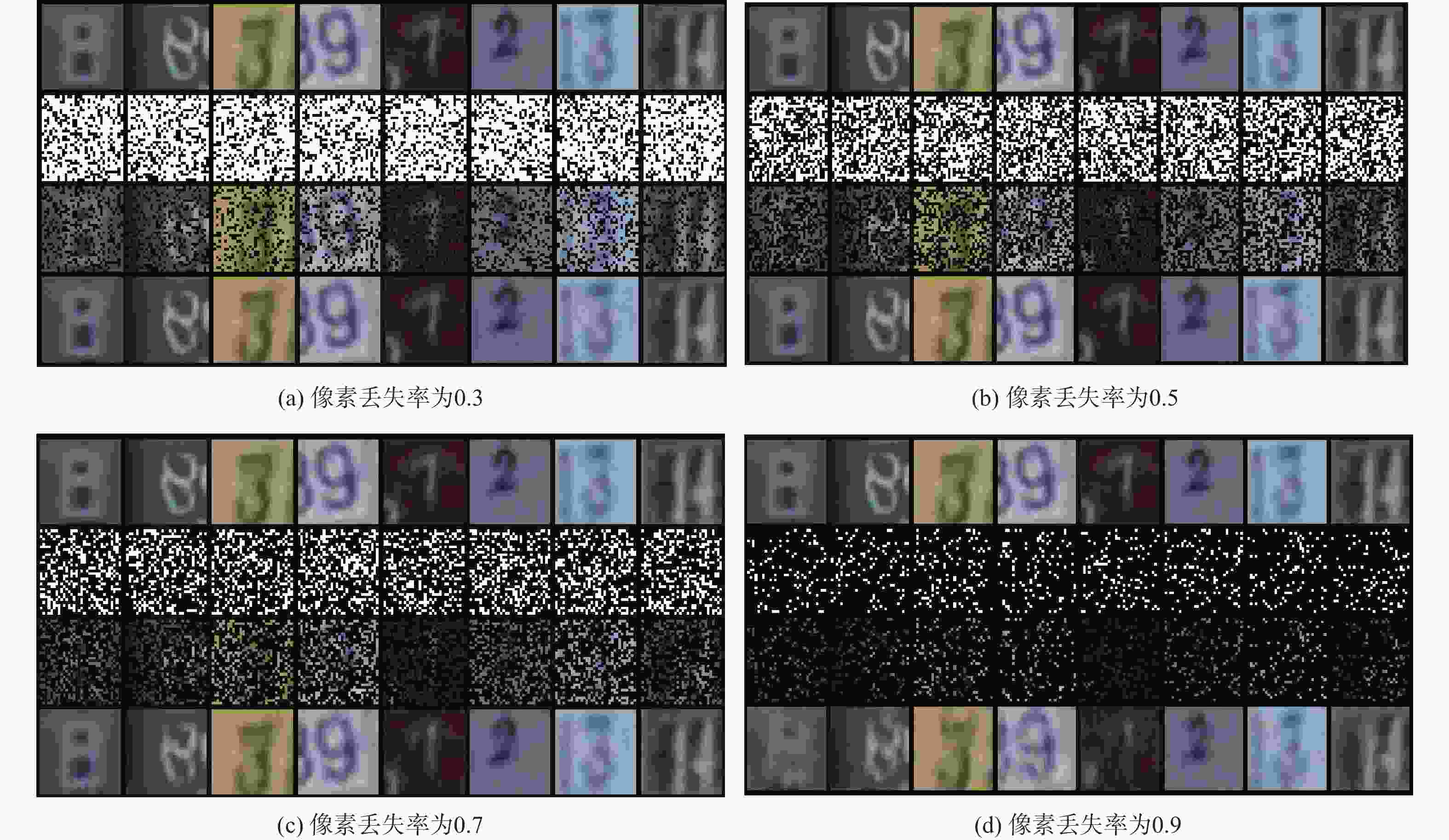
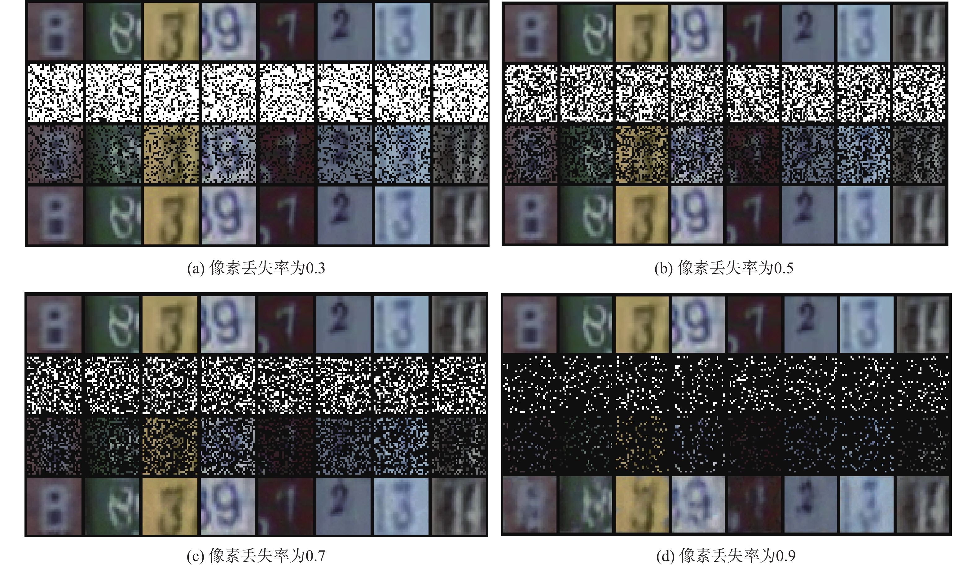
图 5 基于ResSDE-Net的真实世界实拍的数据集SVHN的修复情况
Figure 5. Completed real-world dataset SVHN based on ResSDE-Net
表 1 基本残差块,瓶颈残差块以普通块所构建的24层神经网络架构
Table 1. 24-layer neural network architectures constructed by basic residual blocks, bottleneck residual blocks, and plain blocks
名称 24层基本残差块 24层瓶颈残块 24层普通块 下采样层Conv1 {${3}{ \text{×} }{3,}\;{64,}\;{ {\rm{stride} }\;1}$}; {${4}{\text{×}}{4,64,\;{\rm{stride}}\;2}$}; {${4}{\text{×}}{4,}\;{64,{\rm{stride}}\;2}$} ConcatConv2_x $\left\{ \begin{array}{cc}\text{3}\text{×}\text{3,}\; \left(\text{64, 64}\right)\\ \text{3}\text{×}\text{3,}\; \left(\text{64, 64}\right)\end{array} \right\}$ $\left\{ \begin{array}{c}\begin{array}{cc} \text{1}\text{×}\text{1,}\; \left(\text{64, 64}\right) \\ \text{3}\text{×}\text{3,}\; \left(\text{64, 64}\right) \end{array}\\ \begin{array}{cc} \text{3}\text{×}\text{3,}\; \left(\text{64, 64}\right) \\ \text{1}\text{×}\text{1,}\; \left(\text{64, 64}\right) \end{array}\end{array} \right\}$ $\left\{ \begin{array}{c}\begin{array}{cc} \text{3}\text{×}\text{3,}\; \left(\text{64, 64}\right) \\ \text{3}\text{×}\text{3,}\; \left(\text{64, 64}\right) \end{array}\\ \begin{array}{cc} \text{3}\text{×}\text{3,}\; \left(\text{64, 64}\right) \\ \text{3}\text{×}\text{3,}\; \left(\text{64, 64}\right) \end{array}\end{array} \right\}$ $\left[ \begin{array}{cc}\text{3}\text{×}\text{3,}\; \left(\text{64, 64}\right)\\ \text{3}\text{×}\text{3,}\; \left(\text{64, 64}\right)\end{array} \right]$ ConcatConv3_x $\left\{ \begin{array}{cc}\text{3×3,}\; \left(\text{64, 128}\right)\\ \text{3×3,}\; \left(\text{128, 128}\right)\end{array} \right\}$ $\left\{ \begin{array}{c}\begin{array}{cc} \text{1}\text{×}\text{1,}\; \left(\text{64, 128}\right) \\ \text{3}\text{×}\text{3,}\; \left(\text{128, 128}\right) \end{array}\\ \begin{array}{cc} \text{3}\text{×}\text{3,}\; \left(\text{128, 128}\right) \\ \text{1}\text{×}\text{1,}\; \left(\text{128, 64}\right) \end{array}\end{array} \right\}$ $\left\{ \begin{array}{c}\begin{array}{cc} \text{3}\text{×}\text{3,}\; \left(\text{64, 128}\right) \\ \text{3}\text{×}\text{3,}\; \left(\text{128, 128}\right) \end{array}\\ \begin{array}{cc} \text{3}\text{×}\text{3,}\; \left(\text{128, 64}\right) \\ \text{3}\text{×}\text{3,}\; \left(\text{64, 64}\right) \end{array}\end{array} \right\}$ $\left\{ \begin{array}{cc}\text{3×3,}\; \left(\text{128, 64}\right)\\ \text{3×3,}\; \left(\text{64, 64}\right)\end{array} \right\}$ ConcatConv4_x $\left\{ \begin{array}{cc}\text{3×3,}\; \left(\text{64, 256}\right)\\ \text{3×3,}\; \left(\text{256, 256}\right)\end{array} \right\}$ $\left\{ \begin{array}{c}\begin{array}{cc} \text{1}\text{×}\text{1,}\; \left(\text{64, 256}\right) \\ \text{3}\text{×}\text{3,}\; \left(\text{256, 256}\right) \end{array}\\ \begin{array}{cc} \text{3}\text{×}\text{3,}\; \left(\text{256, 256}\right) \\ \text{1}\text{×}\text{1,}\; \left(\text{256, 64}\right) \end{array}\end{array} \right\}$ $\left\{ \begin{array}{c}\begin{array}{cc} \text{3}\text{×}\text{3,}\; \left(\text{64, 256}\right) \\ \text{3}\text{×}\text{3,}\; \left(\text{256, 256}\right) \end{array}\\ \begin{array}{cc} \text{3}\text{×}\text{3,}\; \left(\text{256, 64}\right) \\ \text{3}\text{×}\text{3,}\; \left(\text{64, 64}\right) \end{array}\end{array} \right\}$ $\left\{ \begin{array}{cc}\text{3}\text{×}\text{3,}\; \left(\text{256, 64}\right)\\ \text{3}\text{×}\text{3,}\; \left(\text{64, 64}\right)\end{array} \right\}$ ConcatConv5_x $\left\{ \begin{array}{cc}\text{3×3,}\; \left(\text{64, 512}\right)\\ \text{3×3,}\; \left(\text{512, 512}\right)\end{array} \right\}$ $\left\{ \begin{array}{c}\begin{array}{cc} \text{1}\text{×}\text{1,}\; \left(\text{64, 512}\right) \\ \text{3}\text{×}\text{3,}\; \left(\text{512, 512}\right) \end{array}\\ \begin{array}{cc} \text{3}\text{×}\text{3,}\; \left(\text{512, 512}\right) \\ \text{1}\text{×}\text{1,}\; \left(\text{512, 64}\right) \end{array}\end{array} \right\}$ $\left\{ \begin{array}{c}\begin{array}{cc} \text{3}\text{×}\text{3,}\; \left(\text{64, 512}\right) \\ \text{3}\text{×}\text{3,}\; \left(\text{512, 512}\right) \end{array}\\ \begin{array}{cc} \text{3}\text{×}\text{3,}\; \left(\text{512, 64}\right) \\ \text{3}\text{×}\text{3,}\; \left(\text{64, 64}\right) \end{array}\end{array} \right\}$ $\left\{ \begin{array}{cc}\text{3×3,}\; \left(\text{512, 64}\right)\\ \text{3×3,}\; \left(\text{64, 64}\right)\end{array} \right\}$ ConcatConv6_x $\left\{ \begin{array}{cc}\text{3}\text{×}\text{3,} \left(\text{64, 1 024}\right)\\ \text{3}\text{×}\text{3,} \left(\text{1 024, 1 024}\right)\end{array} \right\}$ $\left\{ \begin{array}{c}\begin{array}{cc} \text{1}\text{×}\text{1,}\; \left(\text{64, 1 024}\right) \\ \text{3}\text{×}\text{3,} \left(\text{1 024, 1 024}\right) \end{array}\\ \begin{array}{cc} \text{3}\text{×}\text{3,}\; \left(\text{1 024, 1 024}\right) \\ \text{1}\text{×}\text{1,} \left(\text{1 024, 64}\right) \end{array}\end{array} \right\}$ $\left\{ \begin{array}{c}\begin{array}{cc} \text{3}\text{×}\text{3,} \left(\text{64, 1 024}\right) \\ \text{3}\text{×}\text{3,} \left(\text{1 024, 1 024}\right) \end{array}\\ \begin{array}{cc} \text{3}\text{×}\text{3,} \left(\text{1 024, 64}\right) \\ \text{3}\text{×}\text{3,} \left(\text{64, 64}\right) \end{array}\end{array} \right\}$ $\left\{ \begin{array}{cc}\text{3}\text{×}\text{3,}\; \left(\text{1 024, 64}\right)\\ \text{3}\text{×}\text{3,}\; \left(\text{64, 64}\right)\end{array} \right\}$ 全连接层 平均池化,10分类全连接,归化的指数函数Softmax  下载: 导出CSV
表 2 在MNIST 和 SVHN 数据集上的分类和 OOD 检测
Table 2. Classification and OOD detection on MNIST and SVHN datasets
模型方法 分类准确性 TNR at TPR 95% AUROC 检测准确性 AUPR 实验① 实验② 实验① 实验② 实验① 实验② 实验① 实验② In Out 实验① 实验② 实验① 实验② Threshold 99.5±0.0 95.2±0.1 90.1±2.3 66.1±1.9 96.8±0.9 94.4±0.4 92.9±1.1 89.8±0.5 90.0±3.5 96.7±0.2 98.7±0.3 84.6±0.8 DeepEnsemble 99.6 95.4 92.7 66.5 98.0 94.6 94.1 90.1 94.5 97.8 99.1 84.8 MC-dropout 99.5±0.0 95.2±0.1 88.7±0.6 66.9±0.6 95.9±0.4 94.3±0.1 92.0±0.3 89.8±0.2 87.6±2.0 96.7±0.1 98.4±0.1 84.8±0.2 PNs 99.3±0.1 95.0±0.1 90.4±2.8 66.9±2.0 94.1±2.2 89.9±0.6 93.0±1.4 87.4±0.6 73.2±7.3 92.5±0.6 98.0±0.6 82.3±0.9 BBP 99.2±0.3 93.3±0.6 80.5±3.2 42.2±1.2 96.0±1.1 90.4±0.3 91.9±0.9 83.9±0.4 92.6±2.4 96.4±0.2 98.3±0.4 73.9±0.5 p-SGLD 99.3±0.2 94.1±0.5 94.5±2.1 63.5±0.9 95.7±1.3 94.3±0.4 95.0±1.2 87.8±1.2 75.6±5.2 97.9±0.2 98.7±0.2 83.9±0.7 ResSDE-Net 99.6±0.0 95.5±0.2 96.3±1.2 80.6±1.9 99.0±0.3 96.1±0.4 96.3±0.8 91.2±0.5 96.8±0.9 98.3±0.2 99.7±0.1 91.7±0.9 注:加粗数据表示该模型具有最优平均性能。实验①ID数据集为MNIST时,OOD数据集为SVHN;实验②ID数据集为SVHN时,OOD数据集为CIFAR10。
下载: 导出CSV
表 3 MR={0.1,0.3,0.5,0.7,0.9}的ID数据集MNIST、CIFAR10和SVHN
Table 3. ID datasets MNIST, CIFAR10 and SVHN with MR = {0.1, 0.3, 0.5, 0.7, 0.9}
MR MNIST CIFAR10 SVHN cResSDE-Net ResSDE-Net SDE-Net cResSDE-Net ResSDE-Net SDE-Net cResSDE-Net ResSDE-Net SDE-Net 0.1 99.41±0.12 98.82±0.14 98.87±0.06 79.53±0.59 29.11±3.68 23.23±0.25 94.72±0.18 65.27±3.75 62.11±5.55 0.3 99.04±0.17 92.93±0.54 94.98±0.19 77.60±0.46 14.80±2.23 13.11±2.89 94.68±0.13 36.21±3.18 31.22±4.80 0.5 97.64±0.11 74.64±1.52 80.54±0.36 73.70±0.26 12.25±0.98 10.33±0.06 94.46±0.17 24.53±1.78 22.28±2.27 0.7 89.89±0.20 44.02±2.25 49.25±0.11 65.22±0.39 10.92±0.59 10.10±0.08 93.02±0.14 17.80±0.60 19.06±0.47 0.9 38.95±1.49 16.09±1.33 14.56±0.34 40.69±0.71 10.89±0.57 10.18±0.06 71.77±0.30 13.73±0.51 18.18±0.82 注:加粗数据表示该模型具有最优平均性能。
下载: 导出CSV
-
[1] KRIZHEVSKY A, SUTSKEVER I, HINTON G E. Imagenet classification with deep convolutional neural networks[C]//26th Advances in Neural Information Processing Systems. La Jolla: MIT press, 2012: 1097-1105. [2] HE K M, ZHANG X Y, REN S Q, et al. Deep residual learning for image recognition[C]//2016 IEEE Conference on Computer Vision and Pattern Recognition. Piscataway: IEEE Press, 2016: 770-778. [3] 张钹, 朱军, 苏航. 迈向第三代人工智能[J]. 中国科学:信息科学, 2020, 50(9): 1281-1302. doi: 10.1360/SSI-2020-0204ZHANG B, ZHU J, SU H. Toward the third generation of artificial intelligence[J]. Scientia Sinica (Informationis), 2020, 50(9): 1281-1302(in Chinese). doi: 10.1360/SSI-2020-0204 [4] GUO C, PLEISS G, SUN Y, et al. On calibration of modern neural networks[C]//Proceedings of the 34th International Conference on Machine Learning. New York: ACM, 2017: 1321-1330. [5] CHEN R T Q, RUBANOVA Y, BETTENCOURT J, et al. Neural ordinary differential equations[C]//Proceedings of the 32nd International Conference on Neural Information Processing Systems. La Jolla: MIT Press, 2018: 6572–6583. [6] KONG L K, SUN J M, ZHANG C. SDE-Net: Equipping deep neural networks with uncertainty estimates[C]//Proceedings of the 37th International Conference on Machine Learning. New York: ACM, 2020: 5405-5415. [7] ØKSENDAL B. Stochastic differential equations[M]. Berlin: Springer, 2003: 65-84. [8] BASS R F. Stochastic processes[M]. New York: Cambridge University Press, 2011: 6. [9] JEANBLANC M, YOR M, CHESNEY M. Continuous-path random processes: Mathematical prerequisites[M]. Mathematical Methods for Financial Markets. Berlin: Springer, 2009: 3-78. [10] HE K M, ZHANG X Y, REN S Q, et al. Identity mappings in deep residual networks[C]//European Conference on Computer Vision. Berlin: Springer, 2016: 630-645. [11] GORDON J, BRUINSMA W P, FOONG A Y K, et al. Convolutional conditional neural processes[C]//8th International Conference on Learning Representations. Addis Ababa: OpenReview.net, 2020. [12] REZENDE D, MOHAMED S. Variational Inference with Normalizing Flows[C]//Proceedings of the 32nd International Conference on Machine Learning. New York: ACM, 2015: 1530–1538. [13] RAISSI M, KARNIADAKIS G E. Hidden physics models: Machine learning of nonlinear partial differential equations[J]. Journal of Computational Physics, 2018, 357: 125-141. doi: 10.1016/j.jcp.2017.11.039 [14] HE K M, SUN J. Convolutional neural networks at constrained time cost[C]//2015 IEEE Conference on Computer Vision and Pattern Recognition. Piscataway: IEEE Press, 2015: 5353-5360. [15] EMIN O, XAQ P. Skip connections eliminate singularities[C] //International Conference on Learning Representations. Vancouver: OpenReview.net, 2018. [16] LALLEY S P. Stochastic differential equations[D]. Chicago: University of Chicago, 2016: 1-11. [17] 朱军, 胡文波. 贝叶斯机器学习前沿进展综述[J]. 计算机研究与发展, 2015, 52(1): 16-26. doi: 10.7544/issn1000-1239.2015.20140107ZHU J, HU W B. Recent advances in Bayesian machine learning[J]. Journal of Computer Research and Development, 2015, 52(1): 16-26(in Chinese). doi: 10.7544/issn1000-1239.2015.20140107 [18] BLUNDELL C, CORNEBISE J, KAVUKCUOGLU K, et al. Weight uncertainty in neural network[C]//Proceedings of the 32nd International Conference on Machine Learning. New York: ACM, 2015: 1613-1622. [19] MALININ A, GALES M J F. Predictive uncertainty estimation via prior networks[C]//Advances in Neural Information Processing System. La Jolla: MIT Press, 2018: 7047-7058. [20] GAL Y, GHAHRAMANI Z. Dropout as a Bayesian approximation: representing model uncertainty in deep learning[C]//Proceedings of the 33rd International Conference on International Conference on Machine Learning. New York: ACM, 2016: 1050-1059. [21] HENDRYCKS D, GIMPEL K. A baseline for detecting misclassified and out-of-distribution examples in neural networks[C]//International Conference on Learning Representations, arxiv: OpenReview.net, 2016. [22] LI C, CHEN C, CARLSON D, et al. Preconditioned stochastic gradient langevin dynamics for deep neural networks[C]//AAAI Conference on Artificial Intelligence. Palo Alto: AAAI, 2016: 1788-1794. [23] LAKSHMINARAYANAN B, PRITZEL A, BLUNDELL C. Simple and scalable predictive uncertainty estimation using deep ensemble[C]//Advances in Neural Information Processing System. La Jolla: MIT Press, 2017: 6402-6413. -

 下载:
下载:

 点击查看大图

计量
- 文章访问数: 312
- HTML全文浏览量: 21
- PDF下载量: 34
- 被引次数: 0
