融合边界处理机制的学习型麻雀搜索算法

王子恺; 黄学雨; 朱东林; 闫少强; 李权; 郭伟

doi:10.13700/j.bh.1001-5965.2022.0195

融合边界处理机制的学习型麻雀搜索算法

doi: 10.13700/j.bh.1001-5965.2022.0195

1.
江西理工大学信息工程学院，赣州 341000
2.
江西理工大学软件工程学院，南昌 330013
3.
火箭军工程大学作战保障学院，西安 710025

基金项目: 国家重点研发计划(2020YFB1713700)

详细信息

通讯作者:
E-mail：1137753107@qq.com

中图分类号: TP301.6
计量
- 文章访问数: 395
- HTML全文浏览量: 41
- PDF下载量: 19
- 被引次数: 0
出版历程
- 收稿日期: 2022-03-28
- 录用日期: 2022-04-29
- 网络出版日期: 2022-05-10
- 整期出版日期: 2024-01-31

Learning sparrow search algorithm of hybrids boundary processing mechanisms

1.
School of Information Engineering，Jiangxi University of Science and Technology，Ganzhou 341000，China
2.
School of Software Engineering，Jiangxi University of Science and Technology，Nanchang 330013，China
3.
School of Combat Support，Rocket Military Engineering University，Xi’an 710025，China

Funds: National Key R & D Program of China (2020YFB1713700)

More Information

Corresponding author: E-mail：1137753107@qq.com

摘要

摘要:
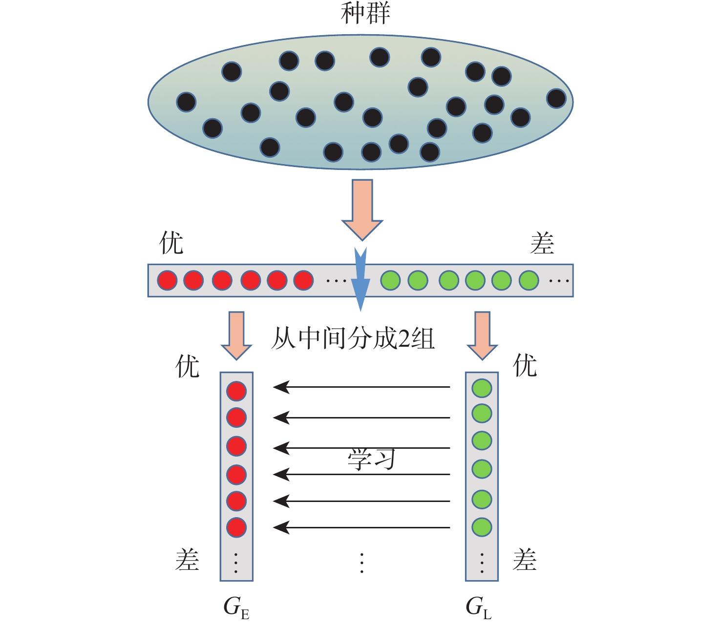
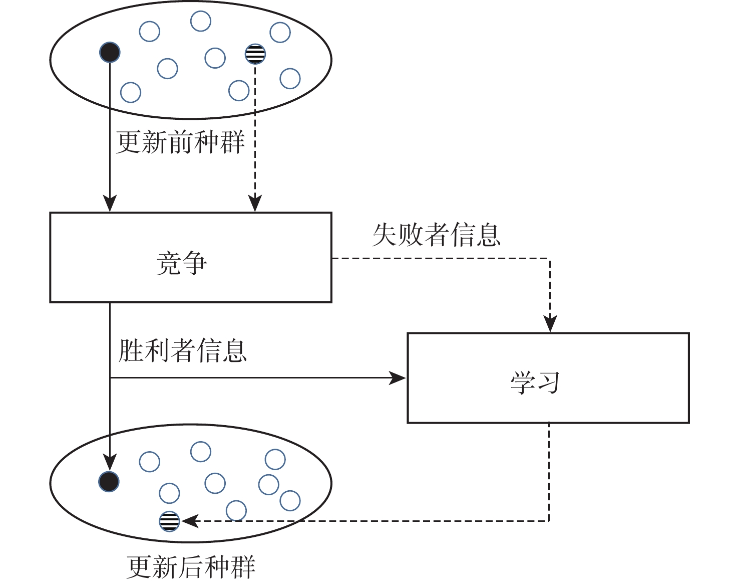
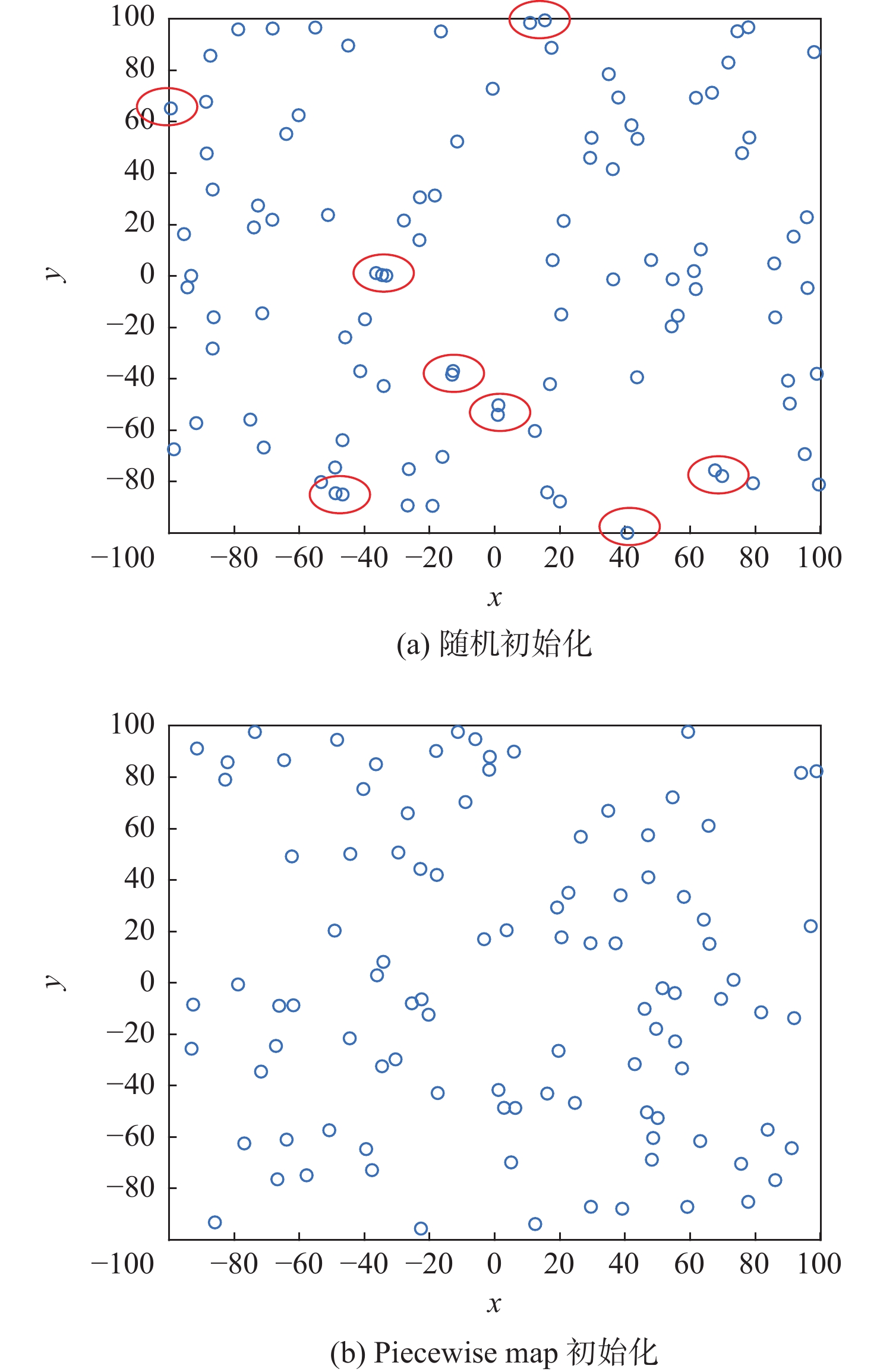
为改善麻雀搜索算法（SSA）初始化阶段种群分布不充分，寻优过程中容易受到局部最优解干扰的不足，提出融合边界处理机制的学习型麻雀搜索算法(HSSA)。使用Piecewise map初始化种群，提高种群的分散程度；使用排序配对学习与竞争学习策略分别更新跟随者和警戒者，确保各代的最优解信息能够引导下一代的位置更新；自适应的警戒者数量使得警戒者作用被强调，提供灵活的应变机制；根据不同阶段的寻优特点制定多策略边界处理机制，保留住种群数量的同时，为超出边界的个体提供更加合理的搜索位置。经过12个基准函数的仿真实验，并借助消融实验、Wilcoxon秩和检验等证明了HSSA在收敛速度上的稳定性和寻优的高效性。
- 麻雀搜索算法 /
- Piecewise map /
- 排序配对学习 /
- 竞争学习 /
- 多策略边界处理
Abstract:
A learning sparrow search algorithm called HSSA that combines a boundary processing mechanism is proposed in order to address the sparrow search algorithm's (SSA) insufficient population distribution during the initialization stage and the optimization process' insufficient interference from local optimal solutions. Using the Piecewise map initializes the population, which improves the population distribution. In order for the position updates of the following generation to be guided by the optimal solution data of each generation, the follower and vigilante are updated individually using the sorted pairing learning and competitive learning procedures. According to the optimization characteristics of different stages, a multi-strategy boundary processing mechanism is formulated. While preserving the population size, it provides a more reasonable search location for individuals beyond the boundary. After 12 simulation experiments of reference functions, the stability of HSSA in convergence speed and the efficiency of optimization are proved by means of ablation experiment and Wilcoxon rank sum test.
- sparrow search algorithm /
- Piecewise map /
- ranking paired learning /
- competitive learning /
- multi-strategy boundary processing mechanisms

HTML全文

图 1 初始种群分布

Figure 1. Distribution of initial population

下载: 全尺寸图片幻灯片

图 2 RPL示意图

Figure 2. Schematic diagram of RPL

下载: 全尺寸图片幻灯片

图 3 竞争学习示意图

Figure 3. Schematic diagram of competitive learning

下载: 全尺寸图片幻灯片

图 4 跟随者阶段边界示意图

Figure 4. Schematic diagram of follower phase boundary processing

下载: 全尺寸图片幻灯片

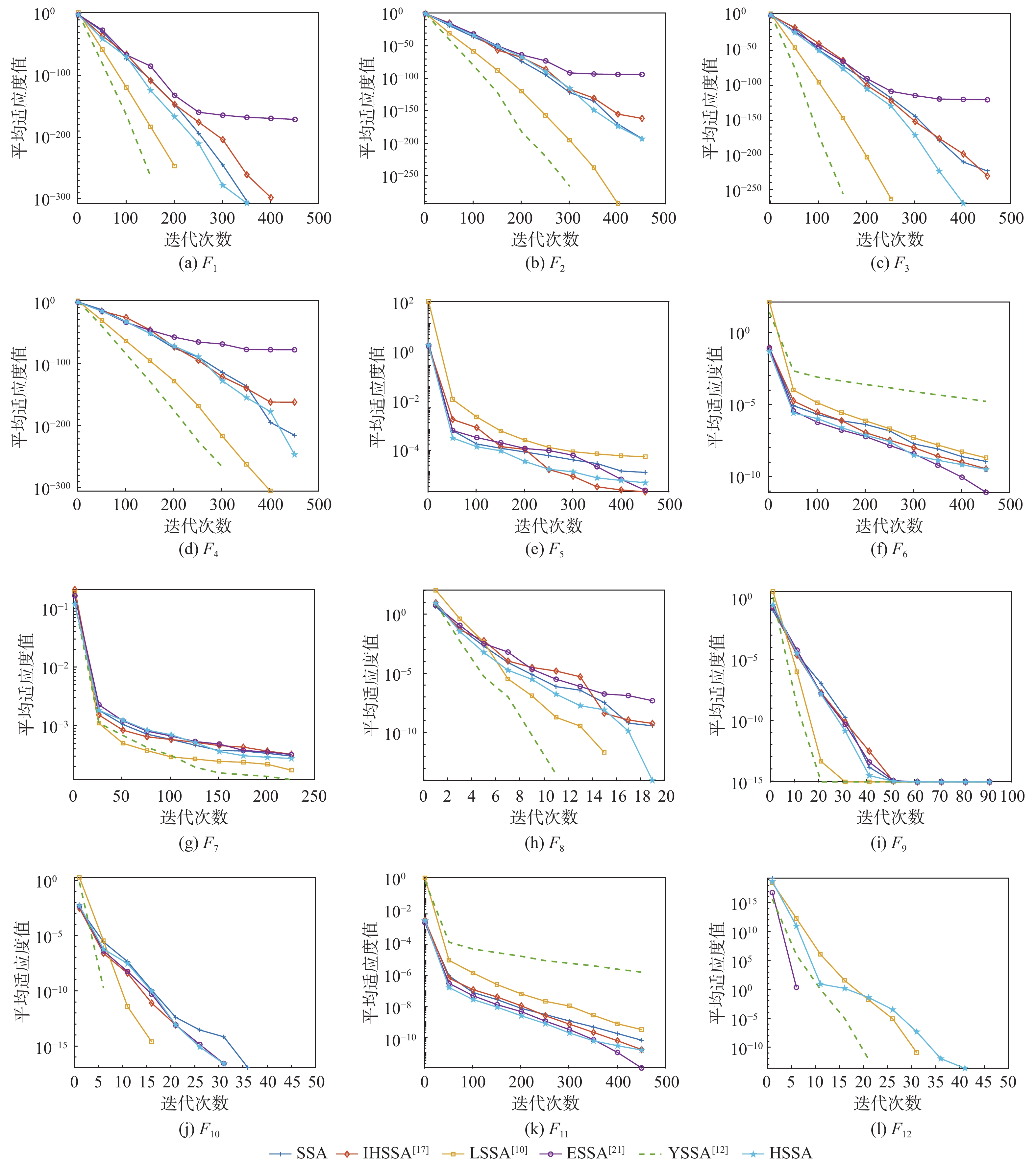
图 5 测试函数收敛曲线

注：对于F₇～F₁₀、F₁₂，6个SSA变体早早地收敛，再展示500代的收敛图不直观，因此，只展示到收敛至最优值附近的代数。

Figure 5. Convergence curve of test functions

下载: 全尺寸图片幻灯片

表 1 算法参数

Table 1. Algorithm parameter

算法	参数	数值
SSA	$ {P}_{{\mathrm{PD}}}$	0.2
	${P}_{{\mathrm{SD}}} $	0.6
	$ \delta $	0.6
IHSSA^[17]	$ {P}_{{\mathrm{PD}}}$	0.2
IHSSA^[17]	$ {P}_{{\mathrm{SD}}} $	0.2
LSSA^[10]	$ {P}_{{\mathrm{PD}}}$	0.2
LSSA^[10]	$ {P}_{{\mathrm{SD}}} $	0.2
ESSA^[21]	$ {P}_{{\mathrm{PD}}}$	0.2
ESSA^[21]	$ {P}_{{\mathrm{SD}}} $	0.2
YSSA^[12]	$ {P}_{{\mathrm{PD}}}$	0.2
YSSA^[12]	$ {P}_{{\mathrm{SD}}} $	0.2
HSSA	$ {P}_{{\mathrm{PD}}} $	0.2
	$ \delta $	0.8
	d	0.3
PSO	$ {c_1} $	1.49445
PSO	$ {c_2} $	1.49445
GWO	$ {a_{{\mathrm{max}}}} $	2
GWO	$ {a_{{\mathrm{min}}}} $	0
BOA	a	0.1
	b	0.025
	c	0.1
	p	0.8

下载: 导出CSV

表 2 基准函数

Table 2. Benchmark function

函数	维度	搜索区域
${F_1}\left( x \right) = \displaystyle\sum_{i = 1}^n x_i^2$	30	[−100,100]
${F_2}\left( x \right) = \displaystyle\sum_{i = 1}^n \left\| {{x_i}} \right\| + \mathop \prod \limits_{i = 1}^n \left\| {{x_i}} \right\|$	30	[−10,10]
${F_3}\left( x \right) = {\displaystyle\sum_{i = 1}^n {\left( {\displaystyle\sum_{j = 1}^i {{x_j}} } \right)} ^2}$	30	[−100,100]
${F_4}\left( x \right) = {\max _i}\left\{ {\left\| {{x_i}} \right\|,1 \leqslant i \leqslant n} \right\}$	30	[−100,100]
${F_5}\left( x \right) =\displaystyle\sum_{i = 1}^{n - 1} \left[ {100{{({x_{i + 1}} - x_i^2)}^2} + {{({x_i} - 1)}^2}} \right]$	30	[−30,30]
$ {F_6}\left( x \right) = \displaystyle\sum_{i = 1}^n {\left( { {{x_i} + 0.5} } \right)^2} $	30	[−100,100]
${F_7}\left( x \right) = \displaystyle\sum_{i = 1}^n {ix_i^4} + {\mathrm{rand}}\left( {0,1} \right)$	30	[−1.28,1.28]
${F_8}\left( x \right) = \displaystyle\sum_{i = 1}^n {\left[ {x_i^2 - 10\cos \left( {2{\text{π}}{x_i}} \right) + 10} \right]} $	30	[−5.12,5.12]
${F_9}\left( x \right) = - 20\exp \left( { - 0.2\sqrt {\dfrac{1}{2}} \displaystyle\sum_{i = 1}^n {x_i^2} } \right) - \exp \left( {\dfrac{1}{n}\displaystyle\sum_{i = 1}^n {\cos \left( {2{\text{π }}{x_i}} \right)} } \right) + 20 + {\mathrm{e}}$	30	[−32,32]
${F_{10}}\left( x \right) = \dfrac{1}{{4\;000}}\displaystyle\sum_{i = 1}^n {x_i^2} - \prod\limits_{i = 1}^n {\cos \left( {\dfrac{{{x_i}}}{{\sqrt i }}} \right)} + 1$	30	[−600,600]
$\begin{gathered} {F_{11}}\left( x \right) = \dfrac{{\text{π }}}{n}\left\{ {10\sin \left( {{\text{π }}{y_1}} \right) + \displaystyle\sum_{i = 1}^{n - 1} {{\left( {{y_i} - 1} \right)}^2}\left[ {1 + 10{{\sin }^2}\left( {{\text{π}}{y_{i + 1}}} \right)} \right] + {{\left( {{y_n} - 1} \right)}^2}} \right\} + \\\qquad\qquad \displaystyle\sum_{i = 1}^n u\left( {{x_i},10,100,4} \right) , {y_i} = 1 + \dfrac{{{x_i} + 1}}{4} , \;\; u\left({x}_{i},a,k,m\right)=\left\{ \begin{array}{l}k{\left({x}_{i}-a\right)}^{m}\qquad{x}_{i} > a\\ 0\qquad\qquad\quad\; -a < {x}_{i} < a\\ k{\left(-{x}_{i}-a\right)}^{m} \quad\;\; {x}_{i} < -a\end{array}\right. \\ \end{gathered} $	30	[−50,50]
$\begin{array}{c}{F_{12}}\left( x \right) = \displaystyle\sum_{i = 1}^n \left( {{\textit{z}}_i^2 - 10\cos \left( {2{\text{π}}{{\textit{z}}_i}} \right) + 10} \right),\end{array}{Z_i} = \left\{ {\begin{array}{l}{{y_i}}\qquad\qquad\qquad {\left\| {{y_i}} \right\|<0.5}\\{\dfrac{{{\rm{round}}\left( {2{y_i}} \right)}}{2}}\qquad {\left\| {{y_i}} \right\| \leqslant 0.5}\end{array}} \right. $	10	[−10¹⁰,10¹⁰]

下载: 导出CSV

表 3 HSSA与SSA变体测试对比

Table 3. Comparison of test HSSA with SSA variants

函数	F₁			F₂			F₃			F₄
函数	平均值	标准差	最优值	平均值	标准差	最优值	平均值	标准差	最优值	平均值	标准差	最优值
SSA	0	0	0	6.62×10⁻²²⁷	0	0	1.85×10⁻²⁵⁴	0	0	8.07×10⁻²⁴¹	0	0
IHSSA^[17]	0	0	0	7.91×10⁻¹⁶³	0	5.34×10⁻¹⁶⁴	8.96×10⁻²⁶⁴	0	0	4.48×10⁻¹⁶³	0	0
LSSA^[10]	0	0	0	0	0	0	0	0	0	0	0	0
ESSA^[21]	1.54×10⁻¹⁷²	0	0	6.54×10⁻⁹⁵	3.52×10⁻⁹⁴	0	1.57×10⁻¹²¹	8.45×10⁻¹²¹	0	8.26×10⁻⁷⁹	4.45×10⁻⁷⁸	0
YSSA^[12]	0	0	0	0	0	0	0	0	0	0	0	0
HSSA	0	0	0	9.28×10⁻²⁵¹	0	0	0	0	0	2.73×10⁻²⁶⁵	0	0

函数	F₅			F₆			F₇			F₈
函数	平均值	标准差	最优值	平均值	标准差	最优值	平均值	标准差	最优值	平均值	标准差	最优值
SSA	1.88×10⁻⁵	3.17×10⁻⁵	1.90×10⁻⁸	5.73×10⁻¹⁰	2.25×10⁻⁹	5.12×10⁻¹⁴	1.54×10⁻⁴	1.09×10⁻⁴	4.65×10⁻⁶	0	0	0
IHSSA^[17]	7.72×10⁻⁷	3.54×10⁻⁶	8.74×10⁻¹²	6.57×10⁻¹¹	1.16×10⁻¹⁰	2.76×10⁻¹³	1.99×10⁻⁴	1.46×10⁻⁴	9.25×10⁻⁶	0	0	0
LSSA^[10]	4.67×10⁻⁵	1.96×10⁻⁴	0	8.10×10⁻¹⁰	2.28×10⁻⁹	3.55×10⁻¹²	8.23×10⁻⁵	6.02×10⁻⁵	5.65×10⁻⁶	0	0	0
ESSA^[21]	2.21×10⁻⁶	7.70×10⁻⁶	2.45×10⁻¹²	9.36×10⁻¹³	1.21×10⁻¹²	1.03×10⁻¹⁴	1.70×10⁻⁴	1.17×10⁻⁴	2.98×10⁻⁵	0	0	0
YSSA^[12]	0	0	0	9.58×10⁻⁶	1.38×10⁻⁵	7.30×10⁻¹⁹	6.84×10⁻⁵	5.03×10⁻⁵	1.34×10⁻⁵	0	0	0
HSSA	2.25×10⁻⁶	5.36×10⁻⁶	1.19×10⁻¹²	4.26×10⁻¹⁰	8.55×10⁻¹⁰	9.79×10⁻¹⁵	1.34×10⁻⁴	8.51×10⁻⁵	1.65×10⁻⁶	0	0	0

函数	F₉			F₁₀			F₁₁			F₁₂
函数	平均值	标准差	最优值	平均值	标准差	最优值	平均值	标准差	最优值	平均值	标准差	最优值
SSA	8.88×10⁻¹⁶	9.86×10⁻³²	8.88×10⁻¹⁶	0	0	0	2.23×10⁻¹¹	6.80×10⁻¹¹	1.52×10⁻¹⁵	0	0	0
IHSSA^[17]	8.88×10⁻¹⁶	9.86×10⁻³²	8.88×10⁻¹⁶	0	0	0	4.23×10⁻¹²	7.02×10⁻¹²	2.85×10⁻¹⁴	0	0	0
LSSA^[10]	8.88×10⁻¹⁶	9.86×10⁻³²	8.88×10⁻¹⁶	0	0	0	7.92×10⁻¹¹	1.87×10⁻¹⁰	1.25×10⁻¹³	0	0	0
ESSA^[21]	8.88×10⁻¹⁶	9.86×10⁻³²	8.88×10⁻¹⁶	0	0	0	1.17×10⁻¹³	2.75×10⁻¹³	2.92×10⁻¹⁷	0	0	0
YSSA^[12]	8.88×10⁻¹⁶	9.86×10⁻³²	8.88×10⁻¹⁶	0	0	0	7.93×10⁻⁷	1.29×10⁻⁶	1.40×10⁻¹⁷	0	0	0
HSSA	8.88×10⁻¹⁶	9.86×10⁻³²	8.88×10⁻¹⁶	0	0	0	1.90×10⁻¹¹	2.11×10⁻¹¹	1.76×10⁻¹⁶	0	0	0

下载: 导出CSV

表 4 HSSA与经典算法测试对比

Table 4. Comparison of test HSSA with classical algorithms

函数	F₁			F₂			F₃			F₄
函数	平均值	标准差	最优值	平均值	标准差	最优值	平均值	标准差	最优值	平均值	标准差	最优值
PSO	7.85×10⁻¹¹	1.72×10⁻¹⁰	4.53×10⁻¹²	5.37×10⁻⁵	1.25×10⁻⁴	1.27×10⁻⁶	5.87	3.40	2.17	2.10×10⁻¹	1.25×10⁻¹	4.70×10⁻²
WOA	5.82×10⁻⁹⁶	1.63×10⁻⁹⁵	2.07×10⁻¹⁰⁵	1.67×10⁻⁵⁷	7.79×10⁻⁵⁷	2.40×10⁻⁶³	1.28×10⁴	7.55×10³	1.02×10³	2.22×10¹	2.73×10¹	2.94×10⁻²
GWO	7.47×10⁻⁴¹	8.36×10⁻⁴¹	2.40×10⁻⁴²	5.44×10⁻²⁴	3.42×10⁻²⁴	1.26×10⁻²⁴	1.03×10⁻¹¹	2.11×10⁻¹¹	1.92×10⁻¹⁴	2.24×10⁻¹⁰	2.92×10⁻¹⁰	4.35×10⁻¹¹
BOA	9.77×10⁻¹²	7.45×10⁻¹³	8.57×10⁻¹²	8.65×10⁻⁶	2.65×10⁻⁵	3.54×10⁻¹⁰	8.89×10⁻¹²	9.75×10⁻¹³	6.52×10⁻¹²	5.11×10⁻⁹	2.67×10⁻¹⁰	4.52×10⁻⁹
TLBO	2.64×10⁻⁸⁵	3.31×10⁻⁸⁵	3.22×10⁻⁸⁶	1.16×10⁻⁴²	5.50×10⁻⁴³	4.67×10⁻⁴³	1.69×10⁻¹⁵	3.61×10⁻¹⁵	8.21×10⁻¹⁷	2.15×10⁻³⁴	7.83×10⁻³⁵	9.95×10⁻³⁵
HSSA	0	0	0	9.28×10⁻²⁵¹	0	0	0	0	0	2.73×10⁻²⁶⁵	0	0

函数	F₅			F₆			F₇			F₈
函数	平均值	标准差	最优值	平均值	标准差	最优值	平均值	标准差	最优值	平均值	标准差	最优值
PSO	3.65×10¹	3.46	1.09	6.46×10⁻¹¹	9.90×10⁻¹¹	2.19×10⁻¹²	1.65×10⁻²	6.24×10⁻²	7.95×10⁻²	5.14×10¹	1.43×10¹	2.39×10¹
WOA	2.68×10¹	0.20	2.63×10¹	4.78×10⁻³	2.50×10⁻³	1.56×10⁻³	1.13×10⁻³	1.23×10⁻³	7.51×10⁻⁵	0	0	0
GWO	2.63×10¹	7.04×10⁻¹	2.52×10¹	2.50×10⁻¹	2.15×10⁻¹	2.20×10⁻⁵	4.74×10⁻⁴	2.71×10⁻⁴	1.30×10⁻⁴	4.00×10⁻¹	1.25	0
BOA	2.89×10¹	2.52×10⁻²	2.89×10¹	5.25	5.34	3.67	2.08×10⁻⁵	2.19×10⁻⁵	1.95×10⁻⁷	1.00×10⁻¹¹	9.53×10⁻¹³	8.13×10⁻¹²
TLBO	1.90×10¹	1.04	1.72×10¹	4.30×10⁻¹⁶	6.62×10⁻¹⁶	1.02×10⁻¹⁷	8.53×10⁻⁴	3.02×10⁻⁴	4.72×10⁻⁴	6.60	5.16	0
HSSA	2.25×10⁻⁶	5.36×10⁻⁶	1.19×10⁻¹²	4.26×10⁻¹⁰	8.55×10⁻¹⁰	9.79×10⁻¹⁵	1.34×10⁻⁴	8.51×10⁻⁵	1.65×10⁻⁶	0	0	0

函数	F₉			F₁₀			F₁₁			F₁₂
函数	平均值	标准差	最优值	平均值	标准差	最优值	平均值	标准差	最优值	平均值	标准差	最优值
PSO	1.04×10⁻¹	3.93×10⁻¹	7.48×10⁻⁷	1.14×10⁻²	1.45×10⁻²	3.30×10⁻¹¹	4.49×10⁻²	8.74×10⁻²	5.87×10⁻¹⁴	1.16×10²⁰	2.95×10¹⁹	5.87×10¹⁹
WOA	3.97×10⁻¹⁵	2.71×10⁻¹⁵	8.88×10⁻¹⁶	4.21×10⁻³	1.29×10⁻²	0	1.91×10⁻¹	1.02	1.84×10⁻⁴	5.92×10⁻¹⁷	3.19×10⁻¹⁶	0
GWO	2.75×10⁻¹⁴	2.71×10⁻¹⁵	2.22×10⁻¹⁴	3.82×10⁻³	7.78×10⁻³	0	1.67×10⁻²	9.03×10⁻³	2.46×10⁻⁶	2.10	3.01	0
BOA	4.45×10⁻⁹	2.24×10⁻¹⁰	3.89×10⁻⁹	1.27×10⁻¹¹	7.39×10⁻¹³	1.12×10⁻¹¹	7.15×10⁻¹	1.14×10⁻¹	5.00×10⁻¹	1.59×10⁷	3.90×10⁷	4.65×10⁴
TLBO	5.98×10⁻¹⁵	1.76×10⁻¹⁵	4.44×10⁻¹⁵	0	0	0	1.05×10⁻¹⁷	1.46×10⁻¹⁷	6.56×10⁻²⁰	5.11	1.03	3.09
HSSA	8.88×10⁻¹⁶	9.86×10⁻³²	8.88×10⁻¹⁶	0	0	0	1.90×10⁻¹¹	2.11×10⁻¹¹	1.76×10⁻¹⁶	0	0	0

下载: 导出CSV

表 5 HSSA与各改进策略消融实验对比

Table 5. Comparion of HSSA with ablation experiments for each improved strategy

函数	F₁			F₂			F₃			F₄
函数	平均值	标准差	最优值	平均值	标准差	最优值	平均值	标准差	最优值	平均值	标准差	最优值
SSA	0	0	0	6.62×10⁻²²⁷	0	0	1.86×10⁻²⁵⁴	0	0	8.07×10⁻²⁴¹	0	0
ISSA1	0	0	0	2.12×10⁻¹⁸⁹	0	0	0	0	0	8.44×10⁻²⁵²	0	0
ISSA2	0	0	0	1.71×10⁻¹⁹⁸	0	0	0	0	0	3.17×10⁻²⁰¹	0	0
ISSA3	0	0	0	1.10×10⁻²⁵⁶	0	0	0	0	0	0	0	0
ISSA4	0	0	0	8.17×10⁻²⁰¹	0	0	0	0	0	5.46×10⁻¹⁹⁵	0	0
ISSA5	0	0	0	1.50×10⁻²¹⁰	0	0	3.72×10⁻²³⁷	0	0	8.45×10⁻²⁴⁹	0	0
ISSA6	0	0	0	3.67×10⁻²²⁵	0	0	2.45×10⁻³⁰⁶	0	0	1.01×10⁻²⁶²	0	0
HSSA	0	0	0	9.28×10⁻²⁵¹	0	0	0	0	0	2.70×10⁻²⁶⁵	0	0

函数	F₅			F₆			F₇			F₈
函数	平均值	标准差	最优值	平均值	标准差	最优值	平均值	标准差	最优值	平均值	标准差	最优值
SSA	1.88×10⁻⁵	3.17×10⁻⁵	1.90×10⁻⁸	5.73×10⁻¹⁰	2.25×10⁻⁹	5.12×10⁻¹⁴	1.54×10⁻⁴	1.09×10⁻⁴	4.60×10⁻⁶	0	0	0
ISSA1	1.86×10⁻⁵	5.01×10⁻⁵	1.20×10⁻⁹	2.03×10⁻¹⁰	4.54×10⁻¹⁰	1.50×10⁻¹³	1.23×10⁻⁴	1.03×10⁻⁴	1.21×10⁻⁵	0	0	0
ISSA2	1.61×10⁻⁵	3.30×10⁻⁵	7.78×10⁻¹⁰	7.68×10⁻¹¹	1.30×10⁻¹⁰	4.92×10⁻¹⁵	1.54×10⁻⁴	1.46×10⁻⁴	7.77×10⁻⁶	0	0	0
ISSA3	5.04×10⁻⁶	8.48×10⁻⁶	2.46×10⁻¹⁰	4.82×10⁻¹⁰	9.39×10⁻¹⁰	6.24×10⁻¹³	1.28×10⁻⁴	1.02×10⁻⁴	1.92×10⁻⁶	0	0	0
ISSA4	4.20×10⁻⁶	4.76×10⁻⁶	3.38×10⁻⁹	9.93×10⁻¹¹	2.32×10⁻¹⁰	1.15×10⁻¹³	1.29×10⁻⁴	8.72×10⁻⁵	5.31×10⁻⁶	0	0	0
ISSA5	1.37×10⁻⁶	1.99×10⁻⁶	1.57×10⁻⁹	3.65×10⁻¹¹	5.76×10⁻¹¹	1.14×10⁻¹⁴	1.58×10⁻⁴	9.62×10⁻⁵	6.21×10⁻⁶	0	0	0
ISSA6	1.61×10⁻⁶	3.81×10⁻⁶	1.13×10⁻¹⁰	8.31×10⁻¹¹	1.57×10⁻¹⁰	6.33×10⁻¹⁶	9.96×10⁻⁵	8.64×10⁻⁵	1.77×10⁻⁶	0	0	0
HSSA	2.25×10⁻⁶	5.36×10⁻⁶	1.19×10⁻¹²	4.26×10⁻¹⁰	8.55×10⁻¹⁰	9.79×10⁻¹⁵	1.34×10⁻⁴	8.51×10⁻⁵	1.65×10⁻⁶	0	0	0

函数	F₉			F₁₀			F₁₁			F₁₂
函数	平均值	标准差	最优值	平均值	标准差	最优值	平均值	标准差	最优值	平均值	标准差	最优值
SSA	8.88×10⁻¹⁶	9.86×10⁻³²	8.88×10⁻¹⁶	0	0	0	2.23×10⁻¹¹	6.80×10⁻¹¹	1.52×10⁻¹⁵	0	0	0
ISSA1	8.88×10⁻¹⁶	9.86×10⁻³²	8.88×10⁻¹⁶	0	0	0	7.17×10⁻¹²	1.91×10⁻¹¹	4.34×10⁻¹⁵	0	0	0
ISSA2	8.88×10⁻¹⁶	9.86×10⁻³²	8.8×10⁻¹⁶	0	0	0	1.54×10⁻¹¹	4.68×10⁻¹¹	9.30×10⁻¹⁶	0	0	0
ISSA3	8.88×10⁻¹⁶	9.86×10⁻³²	8.88×10⁻¹⁶	0	0	0	5.23×10⁻¹¹	1.26×10⁻¹⁰	1.14×10⁻¹⁵	0	0	0
ISSA4	8.88×10⁻¹⁶	9.86×10⁻³²	8.88×10⁻¹⁶	0	0	0	5.26×10⁻¹²	1.43×10⁻¹¹	3.45×10⁻¹⁶	0	0	0
ISSA5	8.88×10⁻¹⁶	9.86×10⁻³²	8.88×10⁻¹⁶	0	0	0	7.27×10⁻¹²	2.20×10⁻¹¹	4.78×10⁻¹⁵	0	0	0
ISSA6	8.88×10⁻¹⁶	9.86×10⁻³²	8.88×10⁻¹⁶	0	0	0	3.36×10⁻¹²	7.56×10⁻¹²	6.77×10⁻¹⁶	0	0	0
HSSA	8.88×10⁻¹⁶	9.86×10⁻³²	8.88×10⁻¹⁶	0	0	0	1.90×10⁻¹¹	2.11×10⁻¹¹	1.76×10⁻¹⁶	0	0	0

下载: 导出CSV

表 6 HSSA与各算法的秩和检验结果

Table 6. Results based on wilcoxon rank test for HSSA with each algorithm

算法	F₁	F₂	F₃	F₄	F₅	F₆	F₇	F₈	F₉	F₁₀	F₁₁	F₁₂
PSO	1.2×10⁻¹²	1.4×10⁻¹¹	1.2×10⁻¹²	6.5×10⁻¹²	3.0×10⁻¹¹	2.2×10⁻²	3.0×10⁻¹¹	1.2×10⁻¹²	1.2×10⁻¹²	1.2×10⁻¹²	1.2×10⁻²	1.2×10⁻¹²
GWO	1.2×10⁻¹²	1.4×10⁻¹¹	1.2×10⁻¹²	6.5×10⁻¹²	3.0×10⁻¹¹	3.0×10⁻¹¹	1.4×10⁻⁷	1.2×10⁻⁵	3.8×10⁻¹³	5.6×10⁻³	3.0×10⁻¹¹	1.5×10⁻⁴
WOA	1.2×10⁻¹²	1.4×10⁻¹¹	1.2×10⁻¹²	6.5×10⁻¹²	3.0×10⁻¹¹	3.0×10⁻¹¹	1.5×10⁻⁵		2.9×10⁻⁷	8.2×10⁻²	3.0×10⁻¹¹	3.3×10⁻¹
TLBO	1.2×10⁻¹²	1.4×10⁻¹¹	1.2×10⁻¹²	6.5×10⁻¹²	3.0×10⁻¹¹	3.0×10⁻¹¹	3.0×10⁻¹¹	1.7×10⁻¹¹	4.5×10⁻¹³		3.0×10⁻¹¹	1.2×10⁻¹²
BOA	1.2×10⁻¹²	1.4×10⁻¹¹	1.2×10⁻¹²	6.5×10⁻¹²	3.0×10⁻¹¹	3.0×10⁻¹¹	2.0×10⁻⁹	1.2×10⁻¹²	1.2×10⁻¹²	1.2×10⁻¹²	3.0×10⁻¹¹	1.2×10⁻¹²
SSA		3.1×10⁻⁴	1.6×10⁻¹	8.2×10⁻¹	7.7×10⁻²	1.6×10⁻²	5.4×10⁻¹				3.9×10⁻¹
IHSSA^[17]		1.4×10⁻¹¹	2.2×10⁻²	3.5×10⁻¹¹	3.0×10⁻⁵	7.3×10⁻³	6.1×10⁻¹				1.3×10⁻¹
LSSA^[10]		3.1×10⁻⁴		1.1×10⁻²	1.5×10⁻¹	1.1×10⁻¹	5.9×10⁻⁴				1.9×10⁻⁴
ESSA^[21]	1.3×10⁻⁵	4.3×10⁻⁶	3.5×10⁻⁷	1.4×10⁻⁷	1.3×10⁻²	1.3×10⁻¹⁰	7.8×10⁻¹				3.8×10⁻⁹
YSSA^[12]		3.1×10⁻⁴		1.1×10⁻²	1.2×10⁻¹²	5.6×10⁻¹⁰	7.7×10⁻⁶				4.6×10⁻⁹

下载: 导出CSV

表 7 Friedman统计结果

Table 7. Friedman statistical results

算法	PSO	GWO	WOA	TLBO	BOA	SSA	IHSSA^[17]	LSSA^[10]	ESSA^[21]	YSSA^[12]	HSSA
综合排名	10.00	8.79	8.54	6.63	8.63	4.19	3.81	3.94	4.27	3.60	3.60

下载: 导出CSV

参考文献(21)

[1]	EBERHART R, KENNEDY J. A new optimizer using particle swarm theory[C]//MHS'95. Proceedings of the Sixth International Symposium on Micro Machine and Human Science. Piscataway: IEEE Press, 2002: 39-43.
[2]	KENNEDY J, EBERHART R. Particle swarm optimization[C]//Proceedings of ICNN'95-International Conference on Neural Networks. Piscataway: IEEE Press, 2002: 1942-1948.
[3]	DORIGO M, GAMBARDELLA L M. Ant colony system: A cooperative learning approach to the traveling salesman problem[J]. IEEE Transactions on Evolutionary Computation, 1997, 1(1): 53-66. doi: 10.1109/4235.585892
[4]	KARABOGA D. An idea based on honey bee swarm for numerical optimization, Technical Report-TR06[R]. Kayseri: Erciyes University, 2005.
[5]	MIRJALILI S, MIRJALILI S M, LEWIS A. Grey wolf optimizer[J]. Advances in Engineering Software, 2014, 69: 46-61. doi: 10.1016/j.advengsoft.2013.12.007
[6]	MIRJALILI S, LEWIS A. The whale optimization algorithm[J]. Advances in Engineering Software, 2016, 95: 51-67. doi: 10.1016/j.advengsoft.2016.01.008
[7]	XUE J, SHEN B. A novel swarm intelligence optimization approach: Sparrow search algorithm[J]. Systems Science & Control Engineering, 2020, 8(1): 22-34.
[8]	吕鑫, 慕晓冬, 张钧, 等. 混沌麻雀搜索优化算法[J]. 北京航空航天大学学报, 2021, 47(8): 1712-1720. doi: 10.13700/j.bh.1001-5965.2020.0298 LYU X, MU X D, ZHANG J, et al. Chaos sparrow search optimization algorithm[J]. Journal of Beijing University of Aeronautics and Astronautics, 2021, 47(8): 1712-1720(in Chinese). doi: 10.13700/j.bh.1001-5965.2020.0298
[9]	毛清华, 张强. 融合柯西变异和反向学习的改进麻雀算法[J]. 计算机科学与探索, 2021, 15(6): 1155-1164. doi: 10.3778/j.issn.1673-9418.2010032 MAO Q H, ZHANG Q. Improved sparrow algorithm combining Cauchy mutation and opposition-based learning[J]. Journal of Frontiers of Computer Science and Technology, 2021, 15(6): 1155-1164(in Chinese). doi: 10.3778/j.issn.1673-9418.2010032
[10]	OUYANG C T, ZHU D L, WANG F Q. A learning sparrow search algorithm[J]. Computational Intelligence and Neuroscience, 2021, 2021: 1-23.
[11]	ZHOU S H, XIE H, ZHANG C C, et al. Wavefront-shaping focusing based on a modified sparrow search algorithm[J]. Optik, 2021, 244: 167516. doi: 10.1016/j.ijleo.2021.167516
[12]	YAN S Q, YANG P, ZHU D L, et al. Improved sparrow search algorithm based on iterative local search[J]. Computational Intelligence and Neuroscience, 2021, 2021: 1-31.
[13]	JOYCE T, HERRMANN J M. A review of no free lunch theorems, and their implications for metaheuristic optimization[J]. Nature-inspired Algorithms and Applied Optimization, 2018, 744: 27-51.
[14]	LI T Y, YORKE J A. The theory of chaotic attractors[M]. Berlin: Springer, 2004: 77-84.
[15]	TIZHOOSH H R. Opposition-based learning: A new scheme for machine intelligence[C]//International Conference on Computational Intelligence for Modelling, Control and Automation and International Conference on Intelligent Agents, Web Technologies and Internet Commerce. Piscataway: IEEE Press, 2006: 695-701.
[16]	OUYANG C T, ZHU D L, QIU Y X. Lens learning sparrow search algorithm[J]. Mathematical Problems in Engineering, 2021, 2021: 1-17.
[17]	WANG Z K, HUANG X Y, ZHU D L. A multistrategy-integrated learning sparrow search algorithm and optimization of engineering problems[J]. Computational Intelligence and Neuroscience, 2022, 2022: 1-21.
[18]	DENG H B, PENG L Z, ZHANG H B, et al. Ranking-based biased learning swarm optimizer for large-scale optimization[J]. Information Sciences, 2019, 493: 120-137. doi: 10.1016/j.ins.2019.04.037
[19]	BALOCHIAN S, BALOOCHIAN H. Social mimic optimization algorithm and engineering applications[J]. Expert Systems with Applications, 2019, 134: 178-191. doi: 10.1016/j.eswa.2019.05.035
[20]	CHENG R, JIN Y C. A competitive swarm optimizer for large scale optimization[J]. IEEE Transactions on Cybernetics, 2015, 45(2): 191-204.
[21]	王振东, 汪嘉宝, 李大海. 一种增强型麻雀搜索算法的无线传感器网络覆盖优化研究[J]. 传感技术学报, 2021, 34(6): 818-828. doi: 10.3969/j.issn.1004-1699.2021.06.016 WANG Z D, WANG J B, LI D H. Study on WSN optimization coverage of an enhanced sparrow search algorithm[J]. Chinese Journal of Sensors and Actuators, 2021, 34(6): 818-828(in Chinese). doi: 10.3969/j.issn.1004-1699.2021.06.016