多策略融合改进的自适应蜉蝣算法

蒋宇飞; 许贤泽; 徐逢秋; 高波

doi:10.13700/j.bh.1001-5965.2022.0492

多策略融合改进的自适应蜉蝣算法

doi: 10.13700/j.bh.1001-5965.2022.0492

武汉大学电子信息学院，武汉 430072

基金项目: 国家自然科学基金(51975422)

详细信息

通讯作者:
E-mail：xxz@whu.edu.cn

中图分类号: TP301.6
计量
- 文章访问数: 515
- HTML全文浏览量: 128
- PDF下载量: 29
- 被引次数: 0
出版历程
- 收稿日期: 2022-06-16
- 录用日期: 2022-09-23
- 网络出版日期: 2022-10-10
- 整期出版日期: 2024-04-29

Multi-strategy fusion improved adaptive mayfly algorithm

School of Electronic Information，Wuhan University，Wuhan 430072，China

Funds: National Natural Science Foundation of China (51975422)

More Information

Corresponding author: E-mail：xxz@whu.edu.cn

摘要

摘要:
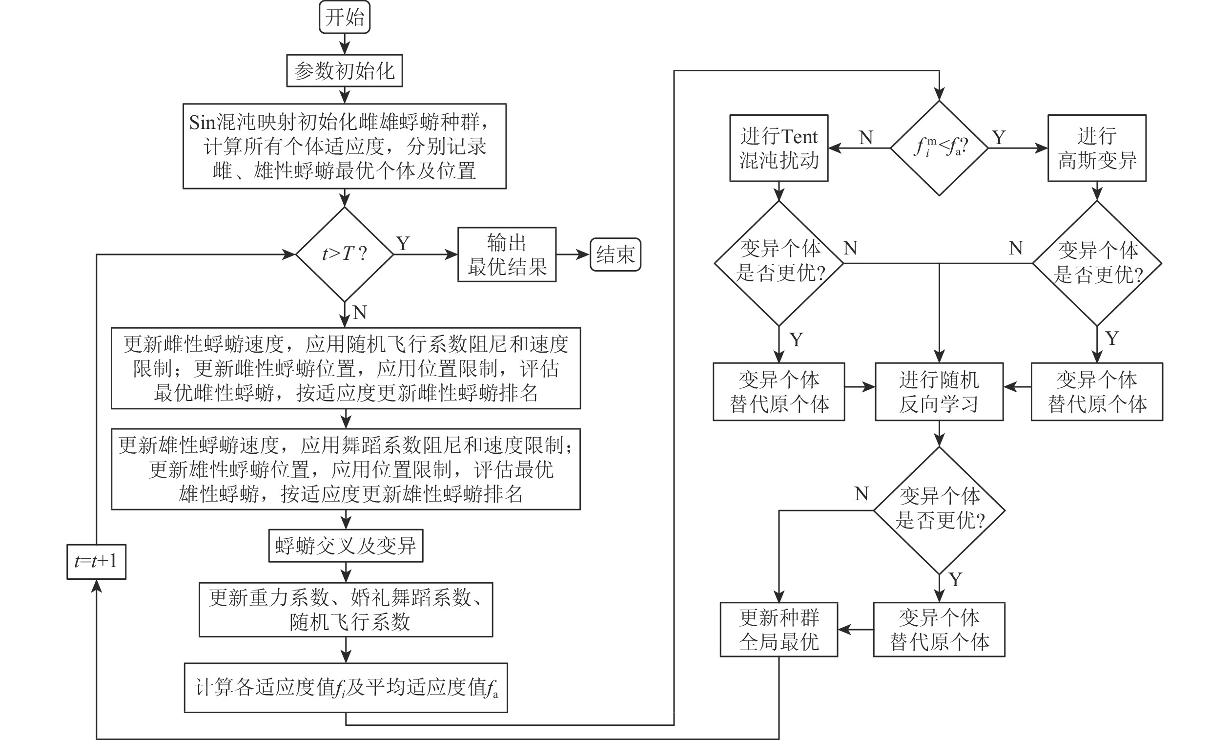
为改进蜉蝣算法全局搜索能力较差、种群多样性较小和自适应能力弱等问题，提出一种多策略融合改进的自适应蜉蝣算法 (MIMA)。采用Sin混沌映射初始化蜉蝣种群，使种群能够均匀分布在解空间中，提高初始种群质量，增强全局搜索能力；引入Tent混沌映射和高斯变异对种群个体进行调节，增加种群多样性的同时调控种群密度，增强局部最优逃逸能力；引入不完全伽马函数，重构自适应动态调节的重力系数，建立全局搜索和局部开发能力之间更好的平衡，进而提升算法收敛精度，有利于提高全局搜索能力；采用随机反向学习 (ROBL) 策略，增强全局搜索能力，提高收敛速度并增强稳定性。利用经典测试函数集进行算法对比，并利用Wilcoxon秩和检验分析算法的优化效果，证明改进的有效性和可靠性。实验结果表明：所提算法与其他算法相比，寻优精度、收敛速度、稳定性都取得了较大提升。
- 蜉蝣算法 /
- 混沌映射 /
- 高斯变异 /
- 自适应动态调节 /
- 随机反向学习
Abstract:
This paper proposes the multi-strategy fusion improved adaptive mayfly algorithm (MIMA), which addresses the shortcomings of the improved mayfly algorithm, including its low adaptive ability, minimal population diversity, and poor global search performance. Firstly, Sin chaos mapping was used to initialize the mayfly population so that the population could be uniformly distributed in the solution space, which improved the initial population quality and enhanced the global search ability. Second, in order to improve the local optimal escape ability, control population density, and boost population diversity, individuals in the population were exposed to Gaussian variation and Tent chaos mapping. Then, the incomplete gamma function was introduced to reconstruct the adaptive dynamic adjustment of gravity coefficients to establish a better balance between global search and local exploitation ability, which in turn improved the convergence accuracy of the algorithm and facilitated the potential of global search to find the optimal solution. Finally, the random opposition-based learning (ROBL) strategy was adopted to enhance the global search ability, improve the convergence speed and enhance the stability. To demonstrate the efficacy and dependability of the four improvement measures, the algorithms were compared using the classical test function set and their optimization effect was examined using the Wilcoxon rank sum test. The experimental results show that compared with other algorithms, the MIMA has better searching accuracy, convergence speed, and stability.
- mayfly algorithm /
- chaotic mapping /
- Gaussian mutation /
- adaptive dynamic adjustment /
- random opposition-based learning

HTML全文

图 1 MIMA算法流程

Figure 1. MIMA Algorithm Flow Chart

下载: 全尺寸图片幻灯片

图 2 测试函数平均收敛曲线

Figure 2. Average convergence curves of test functions

下载: 全尺寸图片幻灯片

表 1 不同$\alpha $值的搜索结果

Table 1. Search results with different ${\boldsymbol{\alpha}} $ values

$\alpha $	平均值	最优值	标准差
1	1.4275×10⁻⁴⁰	5.1651×10⁻⁴⁸	4.4247×10⁻⁴⁰
1.5	2.9239×10⁻⁴⁰	3.7552×10⁻⁴⁷	1.3173×10⁻³⁹
2	1.0435×10⁻³⁹	5.1667×10⁻⁴⁷	4.2855×10⁻³⁹
2.5	3.8230×10⁻³⁹	8.3485×10⁻⁵⁰	2.3260×10⁻³⁸
3	1.7396×10⁻³⁸	2.5809×10⁻⁴⁸	6.7601×10⁻³⁸

下载: 导出CSV

表 2 基准测试函数

Table 2. Benchmark test function

函数公式	维度	搜索空间	$ f_{\min } $
${f_1}\left( x \right) =\textstyle\sum \limits_{i = 1}^n x_i^2$	20	[−100,100]	0
${f_2}\left( x \right) = \textstyle\sum \limits_{i = 1}^n \left\| {{x_i}} \right\| + \mathop \prod \limits_{i = 1}^n \left\| {{x_i}} \right\|$	20	[−10,10]	0
${f_3}\left( x \right) = {\text{max}}\left\{ {\left\| {{x_i}} \right\|} \right\}$	20	[−100,100]	0
${f_4}\left( x \right) = \mathop \sum \limits_{i = 1}^n {\left( {\left\| {{x_i} + 0.5} \right\|} \right)^2}$	20	[−100,100]	0
${f_5}\left( x \right) = \mathop \sum \limits_{i = 1}^n x_i^4 + {\rm{random}}\left[ {0,1} \right)$	20	[−1.28.1.28]	0
${f_6}\left( x \right) = \mathop \sum \limits_{i = 1}^n {\left\| {{x_i}} \right\|^{i + 1}}$	20	[−1,1]	0
${f_7}\left( x \right) = - \mathop \sum \limits_{i = 1}^n \left[ {{x_i}\sin \left( {\sqrt {{x_i}} } \right)} \right]$	20	[−500,500]	−8379.66
${f_8}\left( x \right) = \mathop \sum \limits_{i = 1}^n \left( {x_i^2 - 10\cos \left( {2 \text{π} {x_i}} \right) + 10} \right)$	20	[−5.12,5.12]	0
${f_9}\left( x \right) = - 20\exp \left( { - 0.2\sqrt {\dfrac{1}{n}\mathop \sum \limits_{i = 1}^n x_i^2} } \right) - {\mathrm{exp}}\left(\dfrac{1}{n}\mathop \sum \limits_{i = 1}^n \cos \left( {2 \text{π} {x_i}} \right)\right) + 20 + e$	20	[−32,32]	0
${f_{10}}\left( x \right) = \dfrac{1}{{4\;000}}\mathop \sum \limits_{i = 1}^n x_i^2 - \mathop \prod \limits_{i = 1}^n \cos \left( {\dfrac{{{x_i}}}{{\sqrt i }}} \right) + 1$	20	[−600,600]	0
$ \begin{gathered} {f_{11}}\left( x \right) = \dfrac{ \text{π} }{n}\Biggr[ 10{\mathrm{si}}{{\mathrm{n}}^2}\left( { \text{π} {y_i}} \right) + \textstyle\sum \limits_{i = 1}^{n - 1} {\left( {{y_i} - 1} \right)^2} \Bigr( {1 + 10{\mathrm{si}}{{\mathrm{n}}^2}\left( { \text{π} {y_{i + 1}}} \right)}\Bigr) +\\ {\left( {{y_n} - 1} \right)^2}\Biggr] + \textstyle\sum \limits_{i = 1}^n u\left( {{x_i},10,100,4} \right) \\ \end{gathered} $	20	[−50,50]	0
${f_{12}}\left( x \right) = {\left[0.002 + \sum \limits_{j = 1}^{25} \dfrac{1}{{j + \sum \limits_{i = 1}^2 {{\left( {{x_i} - {a_{ij}}} \right)}^6}}}\right]^{ - 1}}$	2	[−65.53,65.53]	1
${f_{13}}\left( x \right) = \mathop \sum \limits_{i = 1}^{11} {\left[ {{a_i} - \dfrac{{{x_i}\left( {b_i^2 + {b_i}{x_2}} \right)}}{{b_i^2 + {b_i}{x_3} + {x_4}}}} \right]^2}$	4	[−5,5]	3.075 × 10⁻⁴
${f_{14}}\left( x \right) = {\left( {{x_2} - \dfrac{{5.1}}{{4{ \text{π} ^2}}}x_1^2 + \dfrac{5}{ \text{π} }{x_1} - 11} \right)^2} + 10\left( {1 - \dfrac{1}{{8 \text{π} }}} \right){\mathrm{cos}}\;{x_1} + 10$	2	[−5,10]	0.398

下载: 导出CSV

表 3 基准测试函数结果对比

Table 3. Comparison of benchmark test function results

测试函数	平均值
测试函数	MIMA	IMA	PSO	GWO	SCA	IMA2	TCMA
${f_1}$	1.486×10⁻¹⁹²	6.023×10⁻³⁹	2.007	1.945×10⁻⁶⁵	2.717×10⁻⁸	1.229×10⁻⁴⁴	2.310×10⁻⁴⁴
${f_2}$	7.613×10⁻⁹⁸	2.106×10⁻¹⁶	8.188×10⁻¹	2.540×10⁻³⁸	1.844×10⁻⁹	1.576×10⁻²⁴	6.570×10⁻²¹
${f_3}$	9.818×10⁻⁶⁴	2.106×10⁻³	8.653×10⁻¹	3.919×10⁻¹⁶	5.631×10⁻¹	4.224×10⁻⁴	2.976×10⁻⁴
${f_4}$	4.930×10⁻³⁴	1.972×10⁻³³	2.283	4.616×10⁻¹	2.048	0	2.465×10⁻³³
${f_5}$	1.254×10⁻⁴	5.163×10⁻³	5.900×10⁻³	6.322×10⁻⁴	6.508×10⁻³	3.237×10⁻³	4.164×10⁻³
${f_6}$	1.864×10⁻²⁹⁴	7.675×10⁻⁷⁴	4.774×10⁻⁸	2.650×10⁻²²¹	4.803×10⁻⁹	2.972×10⁻⁷²	2.413×10⁻⁷³
${f_7}$	−7.445×10³	−6.881×10³	−5.169×10²	−6.130×10³	−3.234×10³	−8.380×10³	−6.557×10³
${f_8}$	0	2.815	1.909×10¹	4.887×10⁻¹	2.379	3.317×10⁻¹	4.345
${f_9}$	8.882×10⁻¹⁶	1.182	1.840	1.489×10⁻¹⁴	8.627	2.599×10⁻¹⁴	1.614
${f_{10}}$	0	3.780×10⁻²	1.764×10⁻¹	1.776×10⁻³	6.454×10⁻²	2.254×10⁻²	2.146×10⁻¹⁶
${f_{11}}$	2.382×10⁻³²	3.421×10⁻²	4.423×10⁻²	3.328×10⁻²	2.622×10⁻¹	2.408×10⁻³²	5.183×10⁻³
${f_{12}}$	9.980×10⁻¹	9.980×10⁻¹	1.267×10¹	4.131	9.982×10⁻¹	9.980×10⁻¹	9.980×10⁻¹
${f_{13}}$	3.075×10⁻⁴	3.075×10⁻⁴	6.628×10⁻⁴	4.376×10⁻³	9.713×10⁻⁴	1.645×10⁻³	3.075×10⁻⁴
${f_{14}}$	3.979×10⁻¹	3.979×10⁻¹	3.979×10⁻¹	3.979×10⁻¹	3.987×10⁻¹	3.979×10⁻¹	3.979×10⁻¹

测试函数	最优值
测试函数	MIMA	IMA	PSO	GWO	SCA	IMA2	TCMA
${f_{1}}$	5.722×10⁻¹⁹³	8.786×10⁻⁴⁹	6.672×10⁻¹	8.155×10⁻⁶⁸	1.571×10⁻¹⁴	1.468×10⁻⁵¹	2.017×10⁻⁵¹
${f_{2}}$	1.450×10⁻⁹⁹	1.962×10⁻²⁶	5.817×10⁻¹	3.137×10⁻³⁹	6.787×10⁻¹³	2.663×10⁻³⁰	5.440×10⁻²⁷
${f_{3}}$	1.010×10⁻⁹⁷	5.682×10⁻⁵	4.711×10⁻¹	8.026×10⁻¹⁸	6.846×10⁻³	4.710×10⁻⁵	1.529×10⁻⁵
${f_{4}}$	0	0	1.175	1.410×10⁻⁵	1.579	0	0
${f_{5}}$	1.227×10⁻⁷	1.762×10⁻³	9.874×10⁻⁴	1.539×10⁻⁴	4.763×10⁻⁴	1.334×10⁻³	1.468×10⁻³
${f_{6}}$	0	3.927×10⁻⁹³	4.576×10⁻⁹	9.344×10⁻²³¹	9.462×10⁻²²	1.576×10⁻⁹³	1.037×10⁻⁸⁶
${f_{7}}$	−7.926×10³	−7.787×10³	−1.506×10³	−8.067×10³	−3.824×10³	−8.380×10³	−7.432×10³
${f_{8}}$	0	5.684×10⁻¹⁴	8.689	0	5.684×10⁻¹⁴	0	9.950×10⁻¹
${f_{9}}$	8.882×10⁻¹⁶	2.931×10⁻¹⁴	1.015	7.994×10⁻¹⁵	1.877×10⁻⁸	7.994×10⁻¹⁵	6.401×10⁻⁶
${f_{10}}$	0	0	4.317×10⁻²	0	8.378×10⁻¹³	0	0
${f_{11}}$	2.356×10⁻³²	2.356×10⁻³²	7.751×10⁻³	6.514×10⁻³	1.546×10⁻¹	2.356×10⁻³²	2.356×10⁻³²
${f_{12}}$	9.980×10⁻¹	9.980×10⁻¹	1.267×10¹	9.980×10⁻¹	9.980×10⁻¹	9.980×10⁻¹	9.980×10⁻¹
${f_{13}}$	3.075×10⁻⁴	3.075×10⁻⁴	3.166×10⁻⁴	3.075×10⁻⁴	3.436×10⁻⁴	3.075×10⁻⁴	3.075×10⁻⁴
${f_{14}}$	3.979×10⁻¹	3.979×10⁻¹	3.979×10⁻¹	3.979×10⁻¹	3.979×10⁻¹	3.979×10⁻¹	3.979×10⁻¹

测试函数	标准差
测试函数	MIMA	IMA	PSO	GWO	SCA	IMA2	TCMA
${f_{1}}$	0	1.887×10⁻³⁷	7.375×10⁻¹	3.560×10⁻⁶⁵	1.025×10⁻⁷	2.807×10⁻⁴⁴	7.722×10⁻⁴⁴
${f_{2}}$	1.161×10⁻⁹⁷	1.043×10⁻¹⁴	1.153×10⁻¹	2.434×10⁻³⁸	4.370×10⁻⁹	6.994×10⁻²⁴	2.832×10⁻²⁰
${f_{3}}$	4.279×10⁻⁶³	6.188×10⁻³	1.758×10⁻¹	6.989×10⁻¹⁶	1.159	7.688×10⁻⁴	1.555×10⁻⁴
${f_{4}}$	2.415×10⁻³³	7.542×10⁻³³	7.023×10⁻¹	2.647×10⁻¹	2.190×10⁻¹	0	1.121×10⁻³²
${f_{5}}$	1.318×10⁻⁴	2.830×10⁻³	3.497×10⁻³	3.159×10⁻⁴	5.658×10⁻³	1.292×10⁻³	2.459×10⁻³
${f_{6}}$	0	4.000×10⁻⁷³	3.824×10⁻⁸	0	1.413×10⁻⁸	1.590×10⁻⁷¹	8.527×10⁻⁷³
${f_{7}}$	2.102×10²	3.168×10²	2.053×10²	6.476×10²	2.169×10²	1.012×10⁻¹¹	3.688×10²
${f_{8}}$	0	1.888	5.034	1.946	5.766	6.957×10⁻¹	1.441
${f_{9}}$	0	7.940×10⁻¹	5.516×10⁻¹	2.602×10⁻¹⁵	9.000	1.917×10⁻¹⁴	7.649×10⁻¹
${f_{10}}$	0	5.098×10⁻²	6.514×10⁻²	5.066×10⁻³	1.382×10⁻¹	2.578×10⁻²	3.280×10⁻¹⁶
${f_{11}}$	5.825×10⁻³⁴	7.800×10⁻²	3.926×10⁻²	1.549×10⁻²	4.723×10⁻²	1.187×10⁻³³	2.791×10⁻²
${f_{12}}$	7.022×10⁻¹⁷	1.088×10⁻¹⁶	2.139×10⁻¹⁰	4.107	4.398×10⁻⁴	9.065×10⁻¹⁷	1.147×10⁻¹⁶
${f_{13}}$	3.048×10⁻¹⁹	1.870×10⁻¹⁹	2.497×10⁻⁴	7.997×10⁻³	4.014×10⁻⁴	5.003×10⁻³	3.278×10⁻¹⁹
${f_{14}}$	3.331×10⁻¹⁶	3.331×10⁻¹⁶	2.714×10⁻⁵	4.969×10⁻⁵	8.580×10⁻⁴	3.331×10⁻¹⁶	3.331×10⁻¹⁶

下载: 导出CSV

表 4 Wilcoxon秩和检验$p$值

Table 4. $p$-value for Wilcoxon’s rank-sum results

测试函数	IMA	PSO	GWO	SCA	IMA2	TCMA
${f_1}$	3.0199×10⁻¹¹	3.0199×10⁻¹¹	3.0199×10⁻¹¹	3.0199×10⁻¹¹	3.0199×10⁻¹¹	3.0199×10⁻¹¹
${f_2}$	3.0199×10⁻¹¹	3.0199×10⁻¹¹	3.0199×10⁻¹¹	3.0199×10⁻¹¹	3.0199×10⁻¹¹	3.0199×10⁻¹¹
${f_3}$	3.0199×10⁻¹¹	3.0199×10⁻¹¹	3.0199×10⁻¹¹	3.0199×10⁻¹¹	3.0199×10⁻¹¹	3.0199×10⁻¹¹
${f_4}$	7.4577×10⁻⁹	2.3638×10⁻¹²	2.3638×10⁻¹²	2.3638×10⁻¹²	1.6074×10⁻¹	3.0199×10⁻¹¹
${f_5}$	3.0199×10⁻¹¹	3.0199×10⁻¹¹	7.3891×10⁻¹¹	3.0199×10⁻¹¹	3.0199×10⁻¹¹	3.0199×10⁻¹¹
${f_6}$	6.4789×10⁻¹²	6.4789×10⁻¹²	6.4789×10⁻¹²	6.4789×10⁻¹²	6.4789×10⁻¹²	6.4789×10⁻¹²
${f_7}$	2.5306×10⁻⁴	3.0199×10⁻¹¹	9.0632×10⁻⁸	3.0199×10⁻¹¹	2.4306×10⁻¹¹	2.1947×10⁻⁸
${f_8}$	2.5306×10⁻⁴	3.0199×10⁻¹¹	9.0632×10⁻⁸	3.0199×10⁻¹¹	4.5270×10⁻¹²	1.2118×10⁻¹²
${f_9}$	1.2108×10⁻¹²	1.2118×10⁻¹²	2.0341×10⁻¹³	1.2118×10⁻¹²	1.0609×10⁻¹²	1.2118×10⁻¹²
${f_{10}}$	5.7720×10⁻¹¹	1.2118×10⁻¹²	8.1523×10⁻²	1.2118×10⁻¹²	1.6560×10⁻¹¹	2.9112×10⁻²
${f_{11}}$	1.1529×10⁻⁹	2.9729×10⁻¹¹	2.9729×10⁻¹¹	2.9729×10⁻¹¹	3.1958×10⁻⁷	1.4735×10⁻⁷
${f_{12}}$	3.0490×10⁻¹	3.1578×10⁻¹²	1.9881×10⁻¹¹	4.3909×10⁻¹²	7.8056×10⁻¹	6.3241×10⁻¹
${f_{13}}$	NaN	1.2118×10⁻¹²	1.2118×10⁻¹²	1.2118×10⁻¹²	NaN	8.1404×10⁻²
${f_{14}}$	NaN	1.2118×10⁻¹²	1.2118×10⁻¹²	1.2118×10⁻¹²	NaN	NaN
注：NaN表示算法性能相当。

下载: 导出CSV

表 5 消融实验结果

Table 5. Experimental results of ablation

测试函数	平均值
测试函数	IMA	CMA	GMA	MIMA
${f_1}$	6.023×10⁻³⁹	4.459×10⁻¹⁶⁰	8.516×10⁻¹⁵⁶	1.486×10⁻¹⁹²
${f_2}$	2.106×10⁻¹⁶	1.159×10⁻⁹⁴	1.604×10⁻⁸²	7.613×10⁻⁹⁸
${f_3}$	2.106×10⁻³	2.058×10⁻⁶	2.844×10⁻⁵¹	9.818×10⁻⁶⁴
${f_4}$	1.972×10⁻³³	7.396×10⁻³⁴	1.761×10⁻³¹	4.930×10⁻³⁴
${f_5}$	5.163×10⁻³	2.098×10⁻³	1.379×10⁻⁴	1.254×10⁻⁴
${f_6}$	7.675×10⁻⁷⁴	6.998×10⁻²²²	7.204×10⁻²¹⁷	1.864×10⁻²⁹⁴
${f_7}$	−6.881×10³	−7.233×10³	−7.105×10³	−7.445×10³
${f_8}$	2.815	1.678	0	0
${f_9}$	1.182	4.370×10⁻¹⁵	8.882×10⁻¹⁶	8.882×10⁻¹⁶
${f_{10}}$	3.780×10⁻²	0	0	0
${f_{11}}$	3.421×10⁻²	1.662×10⁻²	1.960×10⁻³¹	2.382×10⁻³²
${f_{12}}$	9.980×10⁻¹	9.980×10⁻¹	9.980×10⁻¹	9.980×10⁻¹
${f_{13}}$	3.075×10⁻⁴	1.310×10⁻³	3.075×10⁻⁴	3.075×10⁻⁴
${f_{14}}$	3.979×10⁻¹	3.979×10⁻¹	3.979×10⁻¹	3.979×10⁻¹

测试函数	最优值
测试函数	IMA	CMA	GMA	MIMA
${f_1}$	8.786×10⁻⁴⁹	4.162×10⁻¹⁷³	4.062×10⁻¹⁹⁶	5.722×10⁻¹⁹³
${f_2}$	1.962×10⁻²⁶	3.206×10⁻⁹⁵	4.226×10⁻⁹⁸	1.450×10⁻⁹⁹
${f_3}$	5.682×10⁻⁵	1.443×10⁻²⁴	9.776×10⁻⁹⁸	1.010×10⁻⁹⁷
${f_4}$	0	0	0	0
${f_5}$	1.762×10⁻³	3.955×10⁻⁴	5.288×10⁻⁶	1.227×10⁻⁷
${f_6}$	3.927×10⁻⁹³	1.580×10⁻²³²	7.363×10⁻²²⁹	0
${f_7}$	−7.787×10³	−7.906×10³	−7.906×10³	−7.926×10³
${f_8}$	5.684×10⁻¹⁴	0	0	0
${f_9}$	2.931×10⁻¹⁴	8.882×10⁻¹⁶	8.882×10⁻¹⁶	8.882×10⁻¹⁶
${f_{10}}$	0	0	0	0
${f_{11}}$	2.356×10⁻³²	2.356×10⁻³²	2.404×10⁻³²	2.356×10⁻³²
${f_{12}}$	9.980×10⁻¹	9.980×10⁻¹	9.980×10⁻¹	9.980×10⁻¹
${f_{13}}$	3.075×10⁻⁴	3.075×10⁻⁴	3.075×10⁻⁴	3.075×10⁻⁴
${f_{14}}$	3.979×10⁻¹	3.979×10⁻¹	3.979×10⁻¹	3.979×10⁻¹

测试函数	标准差
测试函数	IMA	CMA	GMA	MIMA
${f_1}$	1.887×10⁻³⁷	2.425×10⁻¹⁵⁹	5.945×10⁻¹⁵⁵	0
${f_2}$	1.043×10⁻¹⁴	1.268×10⁻⁹⁴	1.123×10⁻⁸¹	1.161×10⁻⁹⁷
${f_3}$	6.188×10⁻³	9.700×10⁻⁶	1.240×10⁻⁵⁰	4.279×10⁻⁶³
${f_4}$	7.542×10⁻³³	2.927×10⁻³³	5.428×10⁻³¹	2.415×10⁻³³
${f_5}$	2.830×10⁻³	1.350×10⁻³	1.045×10⁻⁴	1.318×10⁻⁴
${f_6}$	4.000×10⁻⁷³	0	0	0
${f_7}$	3.168×10²	2.789×10²	4.038×10²	2.102×10²
${f_8}$	1.888	2.873	0	0
${f_9}$	7.940×10⁻¹	4.974×10⁻¹⁶	0	0
${f_{10}}$	5.098×10⁻²	0	0	0
${f_{11}}$	7.800×10⁻²	5.627×10⁻²	5.236×10⁻³¹	5.825×10⁻³⁴
${f_{12}}$	1.088×10⁻¹⁶	5.439×10⁻¹⁷	2.259×10⁻¹⁰	7.022×10⁻¹⁷
${f_{13}}$	1.870×10⁻¹⁹	4.371×10⁻³	2.341×10⁻¹⁹	3.048×10⁻¹⁹
${f_{14}}$	3.331×10⁻¹⁶	3.331×10⁻¹⁶	0	3.331×10⁻¹⁶

下载: 导出CSV

参考文献(19)

[1]	RICCI F, ROKACH L, SHAPIRA B. Recommender systems handbook[M]. Berlin: Springer, 2011.
[2]	XUE J K, SHEN B. A novel swarm intelligence optimization approach: Sparrow search algorithm[J]. Systems Science & Control Engineering, 2020, 8(1): 22-34.
[3]	PANDA M, DAS B, PATI B B. Grey wolf optimization for global path planning of autonomous underwater vehicle[C]//Proceedings of the 3rd International Conference on Advanced Informatics for Computing Research. New York: ACM, 2019: 1-6.
[4]	YANG X S. Firefly algorithms for multimodal optimization[C]//Proceedings of the International Symposium on Stochastic Algorithms. Berlin: Springer, 2009: 1-10.
[5]	ZERVOUDAKIS K, TSAFARAKIS S. A mayfly optimization algorithm[J]. Computers & Industrial Engineering, 2020, 145: 106559. doi: 10.1016/j.cie.2020.106559
[6]	张达敏, 徐航, 王依柔, 等. 嵌入Circle映射和逐维小孔成像反向学习的鲸鱼优化算法[J]. 控制与决策, 2021, 36(5): 1173-1180. ZHANG D M, XU H, WANG Y R, et al. Whale optimization algorithm for embedded Circle mapping and one-dimensional oppositional learning based small hole imaging[J]. Control and Decision, 2021, 36(5): 1173-1180(in Chinese).
[7]	胡健, 刘祥敏, 毛伊敏, 等. 基于KD树和混沌蜉蝣优化的并行谱聚类算法[J]. 计算机集成制造系统, 2023, 29(12): 4001-4020. HU J, LIU X M, MAO Y M, et al. Parallel spectral clustering algorithm using KD tree and chaotic mayfly optimization algorithm[J]. Computer Integrated Manufacturing Systems, 2023, 29(12): 4001-4020(in Chinese).
[8]	唐延强, 李成海, 宋亚飞, 等. 自适应变异麻雀搜索优化算法[J]. 北京航空航天大学学报, 2023, 49(3):681-692. TANG Y Q, LI C H, SONG Y F, et al. Adaptive mutation sparrow search optimization algorithm[J]. Journal of Beijing University of Aeronautics and Astronautics, 2023, 49(3):681-692(in Chinese).
[9]	王义, 张达敏, 邹诚诚. 增强全局搜索和自适应蜉蝣算法[J]. 哈尔滨工业大学学报, 2022, 54(11): 137-150. WANG Y, ZHANG D M, ZOU C C. Enhance global search and adaptive mayfly algorithm[J]. Journal of Harbin Institute of Technology, 2022, 54(11): 137-150(in Chinese).
[10]	吕鑫, 慕晓冬, 张钧, 等. 混沌麻雀搜索优化算法[J]. 北京航空航天大学学, 2021, 47(8): 1712-1720. doi: 10.13700/j.bh.1001-5965.2020.0298 LU X, MU X D, ZHANG J, et al. Chaos sparrow search optimization algorithm[J]. Journal of Beijing University of Aeronautics and Astronautics, 2021, 47(8): 1712-1720(in Chinese). doi: 10.13700/j.bh.1001-5965.2020.0298
[11]	张娜, 赵泽丹, 包晓安, 等. 基于改进的Tent混沌万有引力搜索算法[J]. 控制与决策, 2020, 35(4): 893-900. ZHANG N, ZHAO Z D, BAO X A, et al. Gravitational search algorithm based on improved Tent chaos[J]. Control and Decision, 2020, 35(4): 893-900(in Chinese).
[12]	WU K L, YANG M S. Alternative c-means clustering algorithms[J]. Pattern Recognition, 2002, 35(10): 2267-2278. doi: 10.1016/S0031-3203(01)00197-2
[13]	SHI Y. A modified particle swarm optimizer[C]//Proceedings of the IEEE International Conference on Evolutionary Computation. Piscataway: IEEE Press, 1998: 69-73.
[14]	王梦娜, 王秋萍, 王晓峰. 基于Iterative映射和单纯形法的改进灰狼优化算法[J]. 计算机应用, 2018, 38(S2): 16-20. WANG M N, WANG Q P, WANG X F. Improved grey wolf optimization algorithm based on Iterative mapping and simplex method[J]. Journal of Computer Applications, 2018, 38(S2): 16-20(in Chinese).
[15]	TIZHOOSH H R. Opposition-based learning: A new scheme for machine intelligence[C]//Proceedings of the International Conference on International Conference on Computational Intelligence for Modelling, Control & Automation. Piscataway: IEEE Press, 2005: 695-701.
[16]	LONG W, JIAO J, LIANG X, et al. A random opposition-based learning grey wolf optimizer[J]. IEEE Access, 2019, 7: 113810-113825.
[17]	邵瑞凝, 杨博, 束洪春, 等. 基于改进蜉蝣算法的光伏阵列最优重构方法[J]. 电力系统自动化, 2022, 14(11): 142-150. SHAO R N, YANG B, SHU H C, et al. Improved mayfly algorithm for optimal PV array reconfiguration[J]. Automation of Electric Power Systems, 2022, 14(11): 142-150(in Chinese).
[18]	徐焕增, 徐文倩, 孔政敏. 基于Tent混沌序列改进的蜉蝣算法及其应用[J]. 控制工程, 2022, 29(3): 435-440. XU H Z, XU W Q, KONG Z M. Mayfly algorithm based on Tent chaotic sequence and its application[J]. Control Engineering of China, 2022, 29(3): 435-440(in Chinese).
[19]	DERRAC J, GARCIA S, MOLINA D, et al. A practical tutorial on the use of nonparametric statistical tests as a methodology for comparing evolutionary and swarm intelligence algorithms[J]. Swarm & Evolutionary Computation, 2011, 1(1): 3-18.